Introduction to Portfolios

Sukrit Mittal Franklin Templeton Investments

1. Risk and Return: The Core Trade-Off

Finance is not about maximizing return.

It is about choosing how much risk you are willing to tolerate for a given return.

No risk, no reward — but also no free lunches.

This trade-off has been understood for centuries.

The mathematics came later.

What Do We Mean by Return?

Return answers a simple question:

How much did my investment change in value?

But even simple questions deserve precise definitions.

Ambiguity here infects everything downstream.

2. Measuring Return

Let:

\(V(0)\) = initial value
\(V(T)\) = value at the end of the period

The simple return is:

\[ K_V = \frac{V(T)-V(0)}{V(0)} \]

This is the object we will work with throughout this lecture.

Random Nature of Returns

Future returns are unknown today.

Hence, return is modeled as a random variable.

This is not pessimism.

It is intellectual honesty.

3. Expected Return

The expected return summarizes the center of the return distribution.

If \(K_V\) takes values \(k_i\) with probabilities \(p_i\):

\[ \mathbb{E}[K_V] = \sum_{i=1}^n p_i k_i \]

It is a weighted average of possible outcomes.

Interpretation of Expected Return

Not a guaranteed outcome
Not the most likely outcome
A long-run average under repeated trials

Markets do not promise outcomes.

They only offer distributions.

4. Measuring Risk: Variance

Risk is about dispersion, not direction.

The classical measure of risk is variance.

Definition:

\[ \text{Var}(K_V) = \mathbb{E}[(K_V - \mathbb{E}[K_V])^2] \]

Large deviations — up or down — increase variance.

Standard Deviation

The square root of variance is the standard deviation:

\[ \sigma = \sqrt{\text{Var}(K_V)} \]

It has the same units as return.

This makes it easier to interpret and compare.

Criticism of Variance

Variance treats:

Upside surprises
Downside disasters

as equally undesirable.

Investors rarely agree with that philosophy.

This criticism is old — and justified.

5. Downside Risk and Semi-Variance

To focus on losses, we define semi-variance.

Let \(\mu\) be a benchmark (often 0 or the mean).

\[ \text{SemiVar}(K_V) = \mathbb{E}[\max(0, \mu - K_V)^2] \]

Only downside deviations matter.

Why Semi-Variance Is Less Popular

Harder to compute
Harder to optimize
Breaks some elegant mathematics

But conceptually, it is closer to how humans think about risk.

Beauty and realism rarely coexist.

6. Two Securities: Portfolio Return

For weights \(w_1\), \(w_2\) with \(w_1+w_2=1\):

Portfolio return:

\[ K_V = w_1K_1 + w_2K_2 \]

Portfolio expected return:

\[ \mu_V = w_1 \mu_1 + w_2 \mu_2 \]

This is a linear, intuitive relationship.

Two Securities: Portfolio Risk

Portfolio variance:

\[ \sigma_V^2 = w_1^2 \sigma_1^2 + w_2^2 \sigma_2^2 + 2w_1 w_2 \operatorname{Cov}(K_1, K_2) \]

Using correlation \(\rho_{12}\):

\[ \sigma_V^2 = w_1^2 \sigma_1^2 + w_2^2 \sigma_2^2 + 2w_1 w_2 \rho_{12} \sigma_1 \sigma_2 \]

Key insight: Risk depends on co-movement, not individual volatilities alone.

Diversification Mechanism

The portfolio variance formula: \[ \sigma_V^2 = w_1^2 \sigma_1^2 + w_2^2 \sigma_2^2 + 2w_1 w_2 \rho_{12} \sigma_1 \sigma_2 \]
If \(\rho_{12} < 1\), diversification reduces portfolio variance.
The greatest benefit occurs when \(\rho_{12}\) is negative.
Even if both assets are individually risky, their combination can be less risky than either alone. This insight earned Markowitz the Nobel Prize.

Diversification cannot eliminate systematic (market-wide) risk.

Two-asset Theory: Core Idea

Two-Asset Theory states:

Any efficient portfolio composed of two risky assets must lie on a smooth curve in \((\sigma, \mu)\) space.
The curve is parabolic when variance is plotted against weight.
Every investor choosing between only two risky assets will pick a point on this curve based on risk preference.
All efficient portfolios of two risky assets are convex combinations of the two assets.

Two-asset Efficient Frontier

For assets 1 and 2, the efficient frontier is the upper branch of the curve generated by:

\[ \mu(w) = w \mu_1 + (1-w) \mu_2 \]

\[ \sigma^2(w) = w^2 \sigma_1^2 + (1-w)^2 \sigma_2^2 + 2w(1-w) \rho_{12} \sigma_1 \sigma_2 \]

where:

\(w\) is the weight in asset 1 (so \(1-w\) is the weight in asset 2)
\(\mu_1, \mu_2\) are the expected returns
\(\sigma_1, \sigma_2\) are the standard deviations
\(\rho_{12}\) is the correlation between the two assets

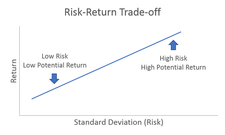
The efficient frontier consists of the portfolios on the upper branch of this curve—those with the highest expected return for a given level of risk.

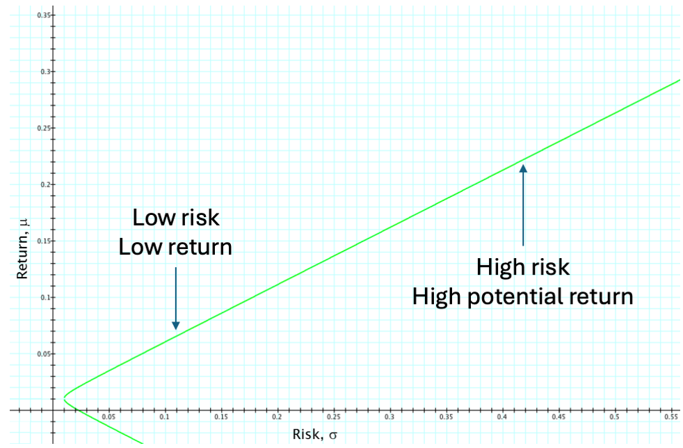
Two-asset Efficient Frontier

Each point corresponds to a value of \(w\) (the weight in asset 1).
The upper part of the curve is efficient—these portfolios offer the best return for a given risk.
The lower part of the curve is dominated—there are always better choices available.
The endpoints correspond to holding 100% of one asset (either asset 1 or asset 2).
Diversification (choosing \(0 < w < 1\)) improves the risk-return trade-off compared to holding a single asset.

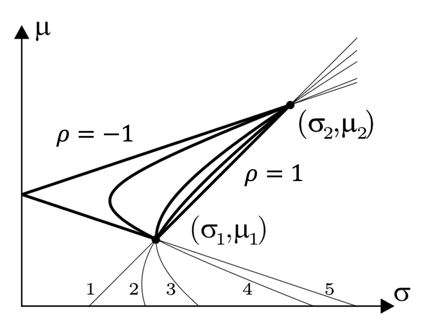
Conditions for the Efficient Set

The conditions for the efficient set (relative to asset 1) are:

If \(\frac{\sigma_1}{\sigma_2} < \rho_{12} \leq 1\), then there exists a portfolio with short selling such that \(\sigma_V < \sigma_1\), but for each portfolio without short selling \(\sigma_V \geq \sigma_1\) (lines 1 and 2).
If \(\rho_{12} = \frac{\sigma_1}{\sigma_2}\), then \(\sigma_V \geq \sigma_1\) for each portfolio (line 3).
If \(-1 \leq \rho_{12} < \frac{\sigma_1}{\sigma_2}\), then there exists a portfolio without short selling such that \(\sigma_V < \sigma_1\) (lines 4 and 5).

These conditions describe when diversification can reduce risk below that of the less risky asset, depending on the correlation and the possibility of short selling.

Minimum Variance Portfolio (MVP)

The Minimum Variance Portfolio (MVP) is the portfolio with the lowest possible risk (variance) for given assets.

The MVP weights are: \[ \boxed{ w_1^* = \frac{\sigma_2^2 - \rho_{12}\sigma_1\sigma_2}{\sigma_1^2 + \sigma_2^2 - 2\rho_{12}\sigma_1\sigma_2}, \quad w_2^* = \frac{\sigma_1^2 - \rho_{12}\sigma_1\sigma_2}{\sigma_1^2 + \sigma_2^2 - 2\rho_{12}\sigma_1\sigma_2} } \]

This gives the unique portfolio with the lowest possible variance for two assets.

How? Minimize \(\sigma_V^2\) subject to \(w_1 + w_2 = 1\).

Derivation Using the Lagrangian

Suppose we have two assets with weights \(w_1\) and \(w_2 = 1 - w_1\). The portfolio variance is: \[ \sigma_V^2 = w_1^2 \sigma_1^2 + (1-w_1)^2 \sigma_2^2 + 2w_1(1-w_1)\rho_{12}\sigma_1\sigma_2 \]

We want to minimize \(\sigma_V^2\) subject to \(w_1 + w_2 = 1\).

Lagrangian Setup

Let \(\lambda\) be the Lagrange multiplier: \[ \mathcal{L}(w_1, w_2, \lambda) = \sigma_V^2 - \lambda(w_1 + w_2 - 1) \]

But since \(w_2 = 1 - w_1\), we can write everything in terms of \(w_1\): \[ \mathcal{L}(w_1, \lambda) = w_1^2 \sigma_1^2 + (1-w_1)^2 \sigma_2^2 + 2w_1(1-w_1)\rho_{12}\sigma_1\sigma_2 - \lambda(w_1 + (1-w_1) - 1) \]

The constraint simplifies to \(w_1 + w_2 - 1 = 0\), which is always satisfied.

Take the Derivative

Set the derivative with respect to \(w_1\) to zero: \[ \frac{\partial \mathcal{L}}{\partial w_1} = 2w_1\sigma_1^2 - 2(1-w_1)\sigma_2^2 + 2(1-2w_1)\rho_{12}\sigma_1\sigma_2 = 0 \]

Expand and solve for \(w_1\): \[ 2w_1\sigma_1^2 - 2\sigma_2^2 + 2w_1\sigma_2^2 + 2\rho_{12}\sigma_1\sigma_2 - 4w_1\rho_{12}\sigma_1\sigma_2 = 0 \]

Group terms: \[ 2w_1(\sigma_1^2 + \sigma_2^2 - 2\rho_{12}\sigma_1\sigma_2) = 2\sigma_2^2 - 2\rho_{12}\sigma_1\sigma_2 \]

Divide both sides by \(2(\sigma_1^2 + \sigma_2^2 - 2\rho_{12}\sigma_1\sigma_2)\): \[ w_1^* = \frac{\sigma_2^2 - \rho_{12}\sigma_1\sigma_2}{\sigma_1^2 + \sigma_2^2 - 2\rho_{12}\sigma_1\sigma_2} \]

Similarly, \[ w_2^* = 1 - w_1^* = \frac{\sigma_1^2 - \rho_{12}\sigma_1\sigma_2}{\sigma_1^2 + \sigma_2^2 - 2\rho_{12}\sigma_1\sigma_2} \]

Second Order Condition

To ensure that the critical point found is a minimum (not a maximum), check the second derivative of \(\sigma_V^2\) with respect to \(w_1\):

\[ \frac{d^2 \sigma_V^2}{d w_1^2} = 2\sigma_1^2 + 2\sigma_2^2 - 4\rho_{12}\sigma_1\sigma_2 \]

This is positive if:

\[ \sigma_1^2 + \sigma_2^2 > 2\rho_{12}\sigma_1\sigma_2 \]

For \(\rho_{12} < 1\), this condition is always satisfied unless the assets are perfectly positively correlated and have identical volatilities. Thus, the solution above gives the minimum variance.

Derivation: Efficient Set Conditions

To determine when diversification reduces portfolio risk below that of the less risky asset, analyze the portfolio variance:

\[ \sigma_V^2 = w_1^2 \sigma_1^2 + w_2^2 \sigma_2^2 + 2w_1 w_2 \rho_{12} \sigma_1 \sigma_2 \]

Assume \(w_1 + w_2 = 1\) and \(0 \leq w_1, w_2 \leq 1\) (no short selling).

Condition for \(\sigma_V < \sigma_1\) without short-selling

\[ 0 \leq w_1^\ast, w_2^\ast \leq 1 \]

\[ 0 \leq \frac{\sigma_2^2 - \rho_{12}\sigma_1\sigma_2}{\sigma_1^2 + \sigma_2^2 - 2\rho_{12}\sigma_1\sigma_2}, \frac{\sigma_1^2 - \rho_{12}\sigma_1\sigma_2}{\sigma_1^2 + \sigma_2^2 - 2\rho_{12}\sigma_1\sigma_2} \leq 1 \]

Since \(\rho_{12} < 1\), the denominator:

\[ \sigma_1^2 + \sigma_2^2 - 2\rho_{12}\sigma_1\sigma_2 > 0 \]

Hence, the numerators need to satisfy:

\[ \sigma_1^2 - \rho_{12}\sigma_1\sigma_2 > 0 \rightarrow \rho_{12} < \frac{\sigma_1}{\sigma_2} \]

\[ \sigma_2^2 - \rho_{12}\sigma_1\sigma_2 > 0 \rightarrow \rho_{12} < \frac{\sigma_2}{\sigma_1} \]

By design, \(\sigma_1 < \sigma_2\). This implies \(\frac{\sigma_1}{\sigma_2} < \frac{\sigma_2}{\sigma_1}\). So, the prevailing condition is:

\[ \rho_{12} < \frac{\sigma_1}{\sigma_2} \]

Summary of Conditions

If \(\rho_{12} < \frac{\sigma_1}{\sigma_2}\): There exists a portfolio (without short selling) with risk less than \(\sigma_1\).
If \(\rho_{12} = \frac{\sigma_1}{\sigma_2}\): The minimum risk equals \(\sigma_1\); no further reduction is possible.
If \(\rho_{12} > \frac{\sigma_1}{\sigma_2}\): Diversification cannot reduce risk below \(\sigma_1\) without short selling.

These conditions define when the efficient set includes portfolios with risk lower than the least risky asset, depending on correlation and asset volatilities.

Derivation: Efficient Frontier Equation for Two Assets

Consider two risky assets with expected returns \(\mu_1\), \(\mu_2\), standard deviations \(\sigma_1\), \(\sigma_2\), and correlation \(\rho_{12}\). Let \(w\) be the weight in asset 1, so \(1-w\) is the weight in asset 2.

Portfolio Expected Return

The expected return of the portfolio is: \[ \mu(w) = w \mu_1 + (1-w) \mu_2 \]

Portfolio Variance

The variance of the portfolio is: \[ \sigma^2(w) = w^2 \sigma_1^2 + (1-w)^2 \sigma_2^2 + 2w(1-w)\rho_{12}\sigma_1\sigma_2 \]

Efficient Frontier Equation

To express the efficient frontier, eliminate \(w\) in favor of \(\mu\):

Solve for \(w\): \[ \mu(w) = w \mu_1 + (1-w) \mu_2 \implies w = \frac{\mu(w) - \mu_2}{\mu_1 - \mu_2} \]

Substitute \(w\) into \(\sigma^2(w)\):

\[ \sigma^2(\mu) = \left[ \frac{\mu - \mu_2}{\mu_1 - \mu_2} \right]^2 \sigma_1^2 + \left[ \frac{\mu_1 - \mu}{\mu_1 - \mu_2} \right]^2 \sigma_2^2 + 2 \left[ \frac{\mu - \mu_2}{\mu_1 - \mu_2} \right] \left[ \frac{\mu_1 - \mu}{\mu_1 - \mu_2} \right] \rho_{12} \sigma_1 \sigma_2 \]

This quadratic equation describes the efficient frontier for all possible portfolios of the two assets.

Interpretation

For each target expected return \(\mu\), the equation gives the minimum achievable risk \(\sigma\).
The upper branch of this curve (highest \(\mu\) for each \(\sigma\)) is the efficient frontier.

Final Takeaways

Risk and return are inseparable: Every investment decision balances potential reward against uncertainty.
Expected return is simple; risk is subtle: Portfolio return combines linearly, but risk depends on asset interactions.
Variance is a useful but imperfect measure: It captures dispersion, but treats gains and losses equally.
Diversification is powered by correlation: Combining assets with less-than-perfect correlation reduces overall risk.
Two assets already reveal deep insights: Even the simplest portfolios illustrate the mathematics and intuition of modern portfolio theory.

This foundation sets the stage for exploring more complex portfolios and the full efficient frontier.