Risk-Free Asset, Preferences, and Optimization

Sukrit Mittal Franklin Templeton Investments

1. Why Add a Risk-Free Asset?

So far, all portfolios involved only risky assets.

That world is incomplete.

In reality, investors can always:

• Park money safely (treasury bills, government bonds)
• Borrow or lend at (approximately) risk-free rates

Ignoring this option distorts everything.

The risk-free asset is not an abstraction.

It is a foundational building block of modern finance.

2. Portfolio with One Risky Asset and One Risk-Free Asset

Let:

• \(R_f\) = risk-free return (constant, deterministic)
• \(R\) = return on a risky asset (random variable)
• \(\mu = \mathbb{E}[R]\) = expected return of risky asset
• \(\sigma = \text{SD}(R)\) = standard deviation of risky asset
• \(w\) = fraction of wealth invested in risky asset
• \(1-w\) = fraction invested in risk-free asset

Portfolio return:

\[ R_p = wR + (1-w)R_f \]

This is the simplest mixed portfolio.

Yet it already contains profound insights.

Expected Return

Taking expectations:

\[ \mathbb{E}[R_p] = w\mathbb{E}[R] + (1-w)R_f = w\mu + (1-w)R_f \]

Rearranging:

\[ \mu_p = R_f + w(\mu - R_f) \]

Interpretation: * Base return: \(R_f\) (certain) * Risk premium: \(w(\mu - R_f)\) (proportional to exposure)

The investor earns a premium only for bearing risk.

Linear in \(w\). Nothing surprising yet.

Risk of the Portfolio

Since \(R_f\) is constant, it has zero variance:

\[ \sigma_p^2 = \text{Var}(wR + (1-w)R_f) = w^2 \text{Var}(R) = w^2\sigma^2 \]

Therefore:

\[ \sigma_p = |w|\sigma \]

Key insight: All risk comes from the risky asset.

The risk-free asset contributes zero to portfolio volatility.

Risk scales linearly with exposure.

Interpretation of Weights

Case 1: \(0 < w < 1\) (Lending) * Invest partially in risky asset * Lend the rest at \(R_f\) * Conservative strategy

Case 2: \(w = 1\) * 100% in risky asset * No borrowing or lending

Case 3: \(w > 1\) (Borrowing) * Borrow at rate \(R_f\) * Invest more than initial wealth in risky asset * Levered strategy

Case 4: \(w < 0\) * Short the risky asset * Invest proceeds in risk-free asset * Extremely conservative

3. Capital Allocation Line (CAL)

From the previous slide: * \(\mu_p = R_f + w(\mu - R_f)\) * \(\sigma_p = |w|\sigma\)

Solve for \(w\) from the second equation:

\[ w = \frac{\sigma_p}{\sigma} \]

Substitute into the first equation:

\[ \mu_p = R_f + \frac{\sigma_p}{\sigma}(\mu - R_f) \]

Rearranging:

\[ \boxed{\mu_p = R_f + \frac{\mu - R_f}{\sigma} \sigma_p} \]

This is the Capital Allocation Line (CAL).

Interpretation of the CAL

The CAL is a straight line in \((\sigma, \mu)\) space.

\[ \mu_p = R_f + \frac{\mu - R_f}{\sigma} \sigma_p \]

• Intercept: \(R_f\) (the risk-free rate)
• Slope: \(\frac{\mu - R_f}{\sigma}\) (reward per unit of risk)

The slope is called the Sharpe Ratio:

\[ \text{Sharpe Ratio} = \frac{\mu - R_f}{\sigma} \]

Interpretation: * Measures excess return per unit of volatility * Higher Sharpe ratio = better risk-adjusted performance * Universal metric for comparing investment strategies

Markets reward efficiency, not bravery.

Graphical Representation

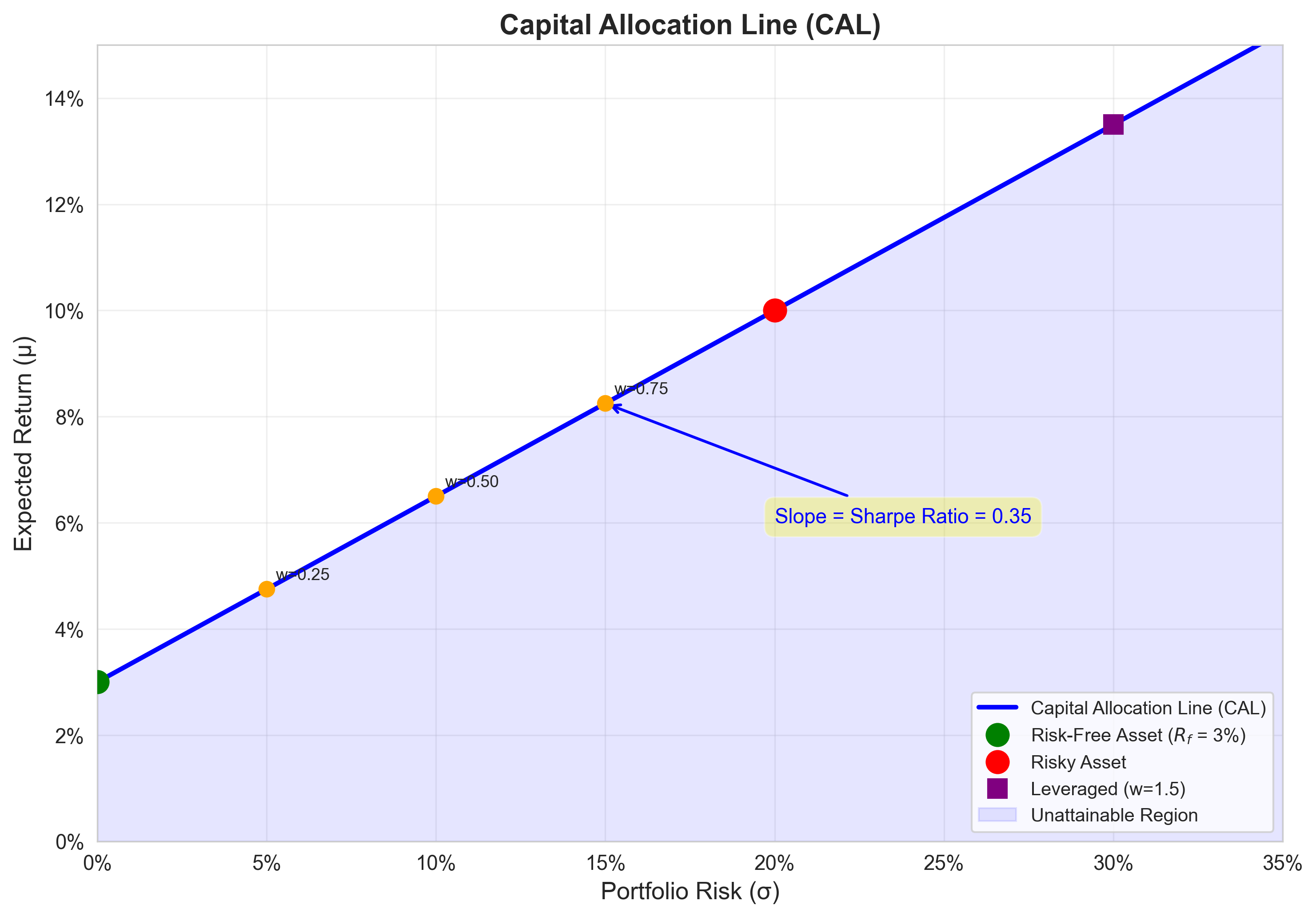
Key observations:

• Every point on the CAL is a portfolio combining \(R_f\) and the risky asset
• Points below the CAL are dominated (achievable with better risk-return)
• Points above the CAL are unattainable (given the assets)
• The CAL extends infinitely in both directions (leverage and short-selling)

The investor’s problem: choose a point on the CAL.

Derivation: Why the CAL is Straight

We derived:

\[ \mu_p = R_f + \frac{\mu - R_f}{\sigma} \sigma_p \]

This is a linear equation in \(\sigma_p\).

Why linearity?

1. Expected return is linear in weights: \(\mu_p = w\mu + (1-w)R_f\)
2. Risk scales linearly with \(w\): \(\sigma_p = w\sigma\)
3. Eliminating \(w\) preserves linearity

Contrast with risky assets only: * Two risky assets form a hyperbola in \((\sigma, \mu)\) space * Adding \(R_f\) “straightens” the efficient frontier

This geometric simplification is the power of the risk-free asset.

4. Many Risky Assets + Risk-Free Asset

When multiple risky assets exist:

1. Step 1: Form the optimal risky portfolio \(M\) from all risky assets
   • This portfolio has expected return \(\mu_M\) and risk \(\sigma_M\)
   • It lies on the efficient frontier of risky assets
2. Step 2: Combine \(M\) with the risk-free asset
   • Choose weight \(w\) in \(M\) and \((1-w)\) in \(R_f\)

The CAL becomes:

\[ \mu_p = R_f + \frac{\mu_M - R_f}{\sigma_M} \sigma_p \]

This line is tangent to the efficient frontier of risky assets.

The Two-Fund Separation Theorem

Theorem: Every investor, regardless of risk preferences, holds: 1. The same optimal risky portfolio \(M\) 2. Some amount of the risk-free asset

Only the mix \((w, 1-w)\) differs across investors.

Implications: * Preferences determine how much risk to take * Preferences do not determine which risky assets to hold * All investors agree on the composition of \(M\)

This is one of the most powerful results in finance.

It justifies index funds and passive investing.

Graphical Illustration: Tangency Portfolio

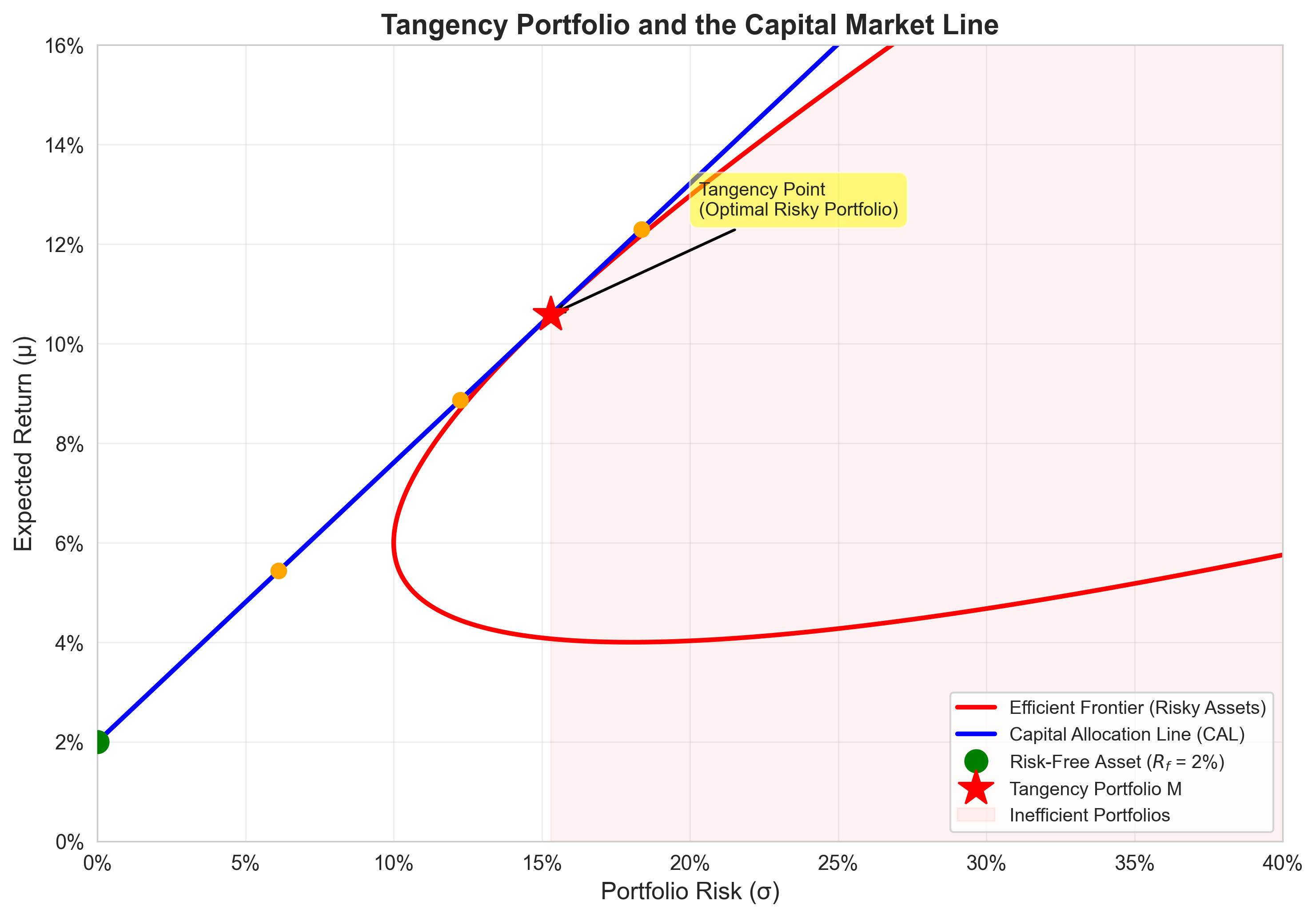
• The tangency portfolio \(M\) maximizes the Sharpe ratio
• The CAL from \(R_f\) through \(M\) dominates all other combinations
• All efficient portfolios lie on this single line

The geometry reveals the economics.

5. Investor Preferences

To choose among portfolios on the CAL, we need a model of preferences.

Finance borrows this machinery from economics.

We assume investors care about:

1. Expected return \(\mu\) (higher is better)
2. Risk \(\sigma\) (lower is better)

These two dimensions define the decision space.

Nothing exotic. Pure rationality.

Mean–Variance Utility Function

Preferences are represented by a utility function:

\[ U(\mu, \sigma^2) = \mu - \frac{\gamma}{2}\sigma^2 \]

Where: * \(U\) = utility (satisfaction level) * \(\mu\) = expected return * \(\sigma^2\) = variance * \(\gamma > 0\) = risk aversion coefficient

Interpretation: * Utility increases with expected return * Utility decreases with variance * \(\gamma\) measures the trade-off rate

This is not psychology.

It is tractable mathematics.

Risk Aversion Parameter \(\gamma\)

The parameter \(\gamma\) determines risk tolerance.

• Large \(\gamma\): High risk aversion
  • Steep penalty for variance
  • Preference for safer portfolios
• Small \(\gamma\): Low risk aversion
  • Mild penalty for variance
  • Willingness to accept more risk
• \(\gamma \to \infty\): Extreme risk aversion
  • Only risk-free asset is acceptable
• \(\gamma \to 0\): Risk neutrality
  • Only expected return matters

Different investors = different \(\gamma\) values.

Same mathematics, different parameters.

6. Indifference Curves

An indifference curve is the set of \((\sigma, \mu)\) pairs yielding equal utility.

Set \(U\) to a constant \(\bar{U}\):

\[ \bar{U} = \mu - \frac{\gamma}{2}\sigma^2 \]

Solve for \(\mu\):

\[ \mu = \bar{U} + \frac{\gamma}{2}\sigma^2 \]

This is a parabola in \((\sigma, \mu)\) space.

Opening upward, with vertex on the \(\mu\)-axis.

Properties of Indifference Curves

1. Upward sloping
   • To compensate for higher risk, higher return is required
   • Slope: \(\frac{d\mu}{d\sigma} = \gamma\sigma > 0\)
2. Convex (increasingly steep)
   • \(\frac{d^2\mu}{d\sigma^2} = \gamma > 0\)
   • Marginal rate of substitution increases with risk
3. Do not intersect
   • Would violate transitivity of preferences
4. Higher curves = higher utility
   • Investors prefer portfolios on higher curves

Geometry replaces psychology.

Graphical Representation

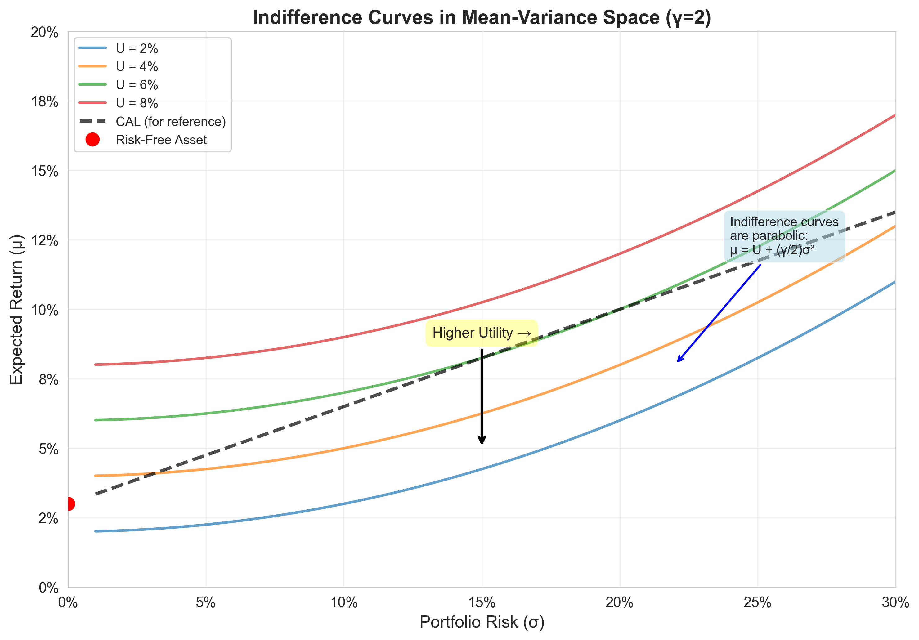
• Each curve represents constant utility
• Curves further northeast = higher utility
• Steepness reflects risk aversion
• Never intersect (consistency of preferences)

The investor seeks the highest attainable curve.

Derivation: Slope of Indifference Curve

From \(U = \mu - \frac{\gamma}{2}\sigma^2\), differentiate implicitly holding \(U\) constant:

\[ dU = 0 = d\mu - \gamma\sigma \, d\sigma \]

Rearranging:

\[ \frac{d\mu}{d\sigma} = \gamma\sigma \]

Interpretation: * The slope is the marginal rate of substitution between risk and return * It increases with \(\sigma\) (convexity) * It increases with \(\gamma\) (risk aversion)

At \(\sigma = 0\): Slope is zero (flat) * No risk, no required compensation

As \(\sigma\) increases: Slope rises * Higher risk demands disproportionately higher return

7. Optimal Portfolio Choice

The investor’s problem:

\[ \max_{w} \quad U(\mu_p, \sigma_p^2) = \mu_p - \frac{\gamma}{2}\sigma_p^2 \]

Subject to: * \(\mu_p = R_f + w(\mu - R_f)\) * \(\sigma_p = w\sigma\)

Substitute into utility:

\[ U(w) = R_f + w(\mu - R_f) - \frac{\gamma}{2}(w\sigma)^2 \]

This is an unconstrained optimization problem in \(w\).

Solving for Optimal Weight

Take the first-order condition:

\[ \frac{dU}{dw} = (\mu - R_f) - \gamma w \sigma^2 = 0 \]

Solve for \(w^*\):

\[ \boxed{w^* = \frac{\mu - R_f}{\gamma \sigma^2}} \]

Interpretation: * Optimal exposure increases with risk premium \((\mu - R_f)\) * Optimal exposure decreases with risk aversion \(\gamma\) * Optimal exposure decreases with variance \(\sigma^2\)

This is the fundamental portfolio allocation formula.

Second-Order Condition

Check the second derivative:

\[ \frac{d^2U}{dw^2} = -\gamma \sigma^2 < 0 \]

Since \(\gamma > 0\) and \(\sigma^2 > 0\), the second derivative is negative.

Therefore, \(w^*\) is a maximum, not a minimum.

The solution is verified.

Numerical Example

Suppose: * \(R_f = 3\%\) * \(\mu = 10\%\) * \(\sigma = 20\%\) * \(\gamma = 2\) (moderate risk aversion)

Optimal weight:

\[ w^* = \frac{0.10 - 0.03}{2 \times 0.20^2} = \frac{0.07}{2 \times 0.04} = \frac{0.07}{0.08} = 0.875 \]

Interpretation: * Invest 87.5% in the risky asset * Invest 12.5% in the risk-free asset

Portfolio characteristics: * \(\mu_p = 0.03 + 0.875(0.10 - 0.03) = 0.09125 = 9.125\%\) * \(\sigma_p = 0.875 \times 0.20 = 0.175 = 17.5\%\)

Sensitivity Analysis

How does \(w^*\) change with parameters?

\[ w^* = \frac{\mu - R_f}{\gamma \sigma^2} \]

1. Higher risk premium \((\mu - R_f)\) → Higher \(w^*\)
   • Better rewards justify more risk
2. Higher risk aversion \(\gamma\) → Lower \(w^*\)
   • More cautious investors take less risk
3. Higher volatility \(\sigma\) → Lower \(w^*\)
   • Riskier assets warrant smaller positions

These relationships are intuitive.

The mathematics merely formalizes common sense.

Graphical Solution: Tangency Condition

The optimal portfolio occurs where:

• An indifference curve is tangent to the CAL

At the tangency point: * Slope of CAL = Slope of indifference curve

CAL slope: \(\frac{\mu - R_f}{\sigma}\)

Indifference curve slope: \(\gamma \sigma_p = \gamma w^* \sigma\)

Setting them equal:

\[ \frac{\mu - R_f}{\sigma} = \gamma w^* \sigma \]

Solving for \(w^*\):

\[ w^* = \frac{\mu - R_f}{\gamma \sigma^2} \]

Geometry and calculus agree.

As they must.

Graphical Representation

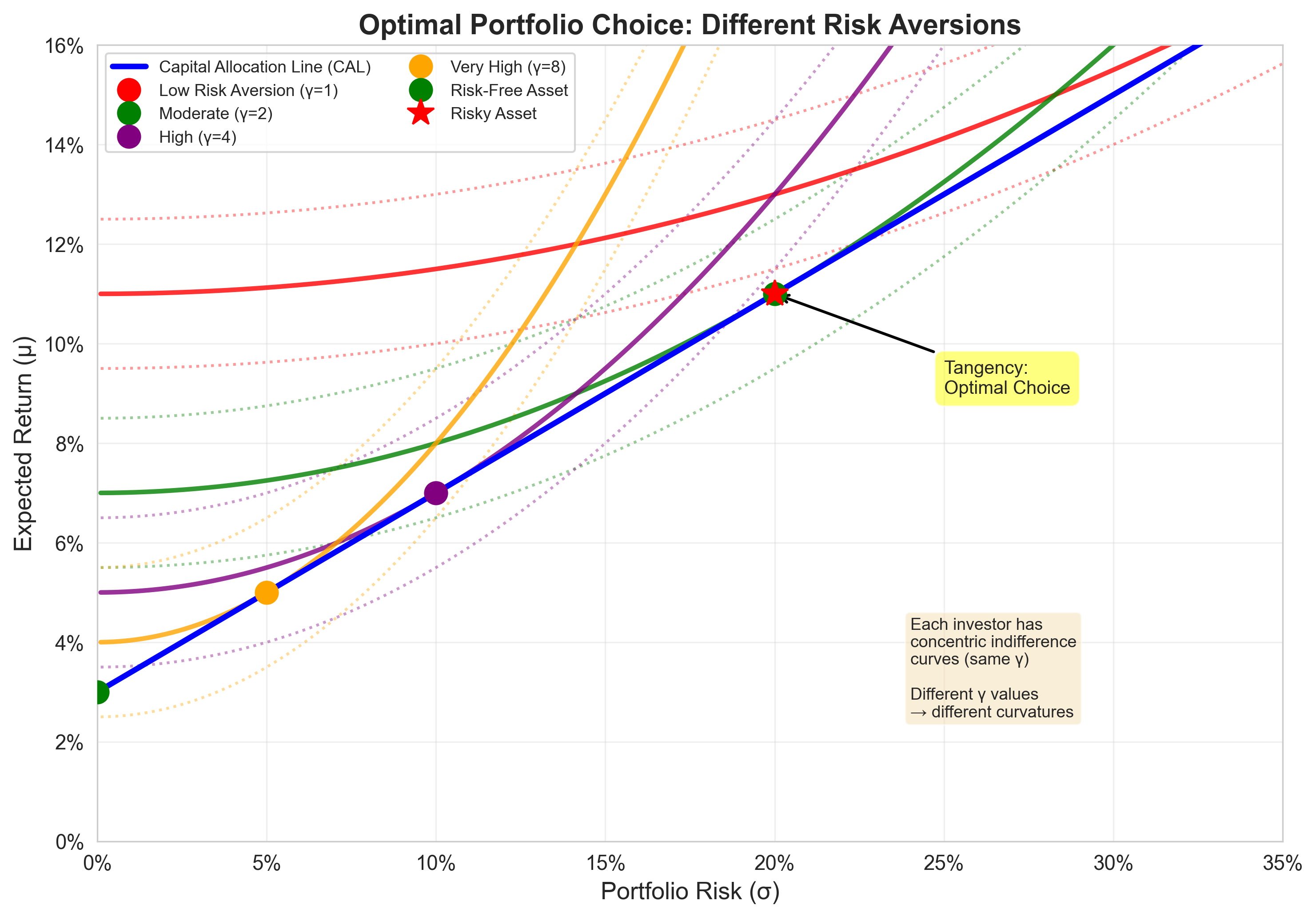
• Different investors have different indifference curves (different \(\gamma\))
• All face the same CAL (same market opportunities)
• Each chooses the tangency point on their indifference curve
• Higher risk aversion → tangency at lower \(\sigma\) (more conservative)

Same risky portfolio.

Different mixing proportions.

This result is deep, old, and still misunderstood.

16. Exercises

Exercise 1: Optimal Portfolio with Risk-Free Asset

Given: * Risk-free rate: \(R_f = 2\%\) * Risky asset expected return: \(\mu = 9\%\) * Risky asset standard deviation: \(\sigma = 15\%\) * Risk aversion: \(\gamma = 3\)

Tasks: 1. Derive the optimal weight \(w^*\) in the risky asset 2. Calculate the expected return and risk of the optimal portfolio 3. How does \(w^*\) change if \(\gamma\) doubles?

Exercise 2: Indifference Curves

An investor has utility function \(U = \mu - 2\sigma^2\).

Tasks: 1. Derive the equation of an indifference curve with utility \(U = 0.05\) 2. Calculate the slope of this curve at \(\sigma = 0.10\) 3. If the CAL has slope \(0.4\), at what value of \(\sigma\) does tangency occur? 4. What is the optimal portfolio return at this tangency?

Exercise 3: Two-Asset Efficient Portfolio

Two assets have: * \(\mu_1 = 6\%\), \(\sigma_1 = 12\%\) * \(\mu_2 = 14\%\), \(\sigma_2 = 25\%\) * \(\rho_{12} = 0.2\)

Tasks: 1. Find the weights for a portfolio with target return \(\mu_p = 10\%\) 2. Calculate the variance of this portfolio 3. Find the minimum variance portfolio (no target return) 4. Compare the two portfolios’ risk levels

Exercise 4: Sharpe Ratio Maximization

Prove that the tangency portfolio (from \(R_f\) to the efficient frontier) maximizes the Sharpe ratio among all risky portfolios.

Hint: Use the fact that at tangency, the slope of the CAL equals the slope of the efficient frontier.

Tasks: 1. Set up the optimization problem 2. Use Lagrange multipliers to find the tangency portfolio 3. Show that this portfolio has the highest Sharpe ratio 4. Interpret the result economically

Final Takeaways

• Adding a risk-free asset transforms portfolio theory:
  • Efficient frontier becomes a straight line (CAL)
  • All investors hold the same risky portfolio (two-fund separation)
  • Only the risk-free/risky mix differs across investors
• Preferences formalize decision-making:
  • Mean-variance utility captures risk-return trade-offs
  • Indifference curves visualize preferences geometrically
  • Risk aversion determines portfolio allocation
• Optimal choice is a tangency condition:
  • Graphically: indifference curve tangent to CAL
  • Analytically: \(w^* = \frac{\mu - R_f}{\gamma \sigma^2}\)
  • Same intuition, different representations
• Lagrange multipliers are unavoidable:
  • Every constrained optimization uses this method
  • Multipliers have economic interpretations (shadow prices)
  • Foundation for all advanced portfolio theory
• Theory guides practice:
  • These results justify index funds and passive strategies
  • Risk parity, factor models, and dynamic allocation all build on this foundation
  • Mathematics reveals economic truth

Next lecture: We extend this framework to multi-asset portfolios and derive the full efficient frontier.