Portfolios of Multiple Assets
Sukrit Mittal Franklin Templeton Investments
Outline
- From two assets to many
- Portfolio return and risk (general case)
- Geometry of diversification
- Three risky securities
- Minimum variance portfolio (MVP)
- Minimum variance set and line
- Introducing the market portfolio
- Exercises
1. From Two Assets to Many
The two-asset case taught us geometry.
The multi-asset case teaches us structure.
Nothing fundamentally new appears.
What changes is notation—and discipline.
Why This Matters
Real portfolios:
- Contain many assets
- Are constrained by budgets
- Must be optimized systematically
- The geometry becomes higher-dimensional
- But the economic principles remain unchanged
2. Portfolio Return: General Case
Let:
- \(n\) risky assets
- returns \(R = (R_1, \dots, R_n)^\top\)
- weights \(w = (w_1, \dots, w_n)^\top\)
Portfolio return:
\[ R_p = w^\top R \]
Budget constraint:
\[ \sum_{i=1}^n w_i = 1 \]
Expected Return
Let \(\mu = \mathbb{E}[R]\) be the vector of expected returns.
Then:
\[ \mathbb{E}[R_p] = w^\top \mu = \sum_{i=1}^n w_i \mu_i \]
Interpretation:
- Expected portfolio return is a weighted average
- Weights are portfolio allocations
- This is perfectly linear
Example: Three-Asset Portfolio
Suppose: * Asset 1: \(\mu_1 = 8\%\), \(w_1 = 0.3\) * Asset 2: \(\mu_2 = 12\%\), \(w_2 = 0.5\) * Asset 3: \(\mu_3 = 15\%\), \(w_3 = 0.2\)
Portfolio expected return: \[ \mu_p = 0.3(0.08) + 0.5(0.12) + 0.2(0.15) = 0.024 + 0.060 + 0.030 = 0.114 = 11.4\% \]
3. Portfolio Risk: Variance
Let \(\Sigma\) be the covariance matrix:
\[ \Sigma_{ij} = \text{Cov}(R_i, R_j) \]
Portfolio variance:
\[ \sigma_p^2 = w^\top \Sigma w = \sum_{i=1}^n \sum_{j=1}^n w_i w_j \Sigma_{ij} \]
This single quadratic form drives modern portfolio theory.
Expanded form:
\[ \sigma_p^2 = \sum_{i=1}^n w_i^2 \sigma_i^2 + \sum_{i=1}^n \sum_{j \neq i} w_i w_j \text{Cov}(R_i, R_j) \]
- First term: individual variances weighted by squared weights
- Second term: all pairwise covariances
The cross terms dominate for large \(n\).
Properties of the Covariance Matrix
Symmetric: \(\Sigma_{ij} = \Sigma_{ji}\)
- Covariance is symmetric by definition
Positive semi-definite: \(w^\top \Sigma w \geq 0\) for all \(w\)
- Variance cannot be negative
- Critical for optimization
Invertible (usually): \(\Sigma^{-1}\) exists
- Required for many portfolio formulas
- Fails only in degenerate cases
Numerical Example: Three-Asset Covariance
Consider the covariance matrix:
\[ \Sigma = \begin{pmatrix} 0.04 & 0.01 & 0.02 \\ 0.01 & 0.09 & 0.03 \\ 0.02 & 0.03 & 0.16 \end{pmatrix} \]
For \(w = (0.3, 0.5, 0.2)^\top\):
\[ \sigma_p^2 = w^\top \Sigma w = 0.3^2(0.04) + 0.5^2(0.09) + 0.2^2(0.16) = 0.0439 \]
Therefore: \(\sigma_p = \sqrt{0.0439} = 20.95\%\)
The diversification benefit is embedded in the covariances.
4. Geometry of Diversification
Expected return is linear in \(w\). Variance is quadratic in \(w\).
Why Diversification Works
As \(n\) increases:
- Number of variance terms: \(n\)
- Number of covariance terms: \(n(n-1)\)
For equally weighted portfolios (\(w_i = 1/n\)):
\[ \sigma_p^2 = \frac{1}{n} \bar{\sigma}^2 + \frac{n-1}{n} \bar{\text{Cov}} \]
Where: * \(\bar{\sigma}^2\) = average variance * \(\bar{\text{Cov}}\) = average covariance
As \(n \to \infty\):
\[ \sigma_p^2 \to \bar{\text{Cov}} \]
Interpretation: Diversification eliminates idiosyncratic risk. Only systematic (correlated) risk remains.
Numerical Example: Diversification Benefits
Consider \(n\) assets with: * Individual variance: \(\sigma^2 = 0.09\) (30% volatility) * Average pairwise correlation: \(\bar{\rho} = 0.35\) * Hence, average pairwise covariance: \(\bar{\text{Cov}} = 0.0315\)
Equally weighted portfolio variance:
| \(n\) | \(\sigma_p^2\) | \(\sigma_p\) | Reduction |
|---|---|---|---|
| 1 | 0.0900 | 30.00% | 0% |
| 5 | 0.0432 | 20.78% | 31% |
| 10 | 0.0373 | 19.33% | 36% |
| 50 | 0.0326 | 18.07% | 40% |
| \(\infty\) | 0.0315 | 17.75% | 41% |
Risk decreases rapidly at first, then asymptotes. This is the power—and limit—of diversification.
Diversification Benefits:
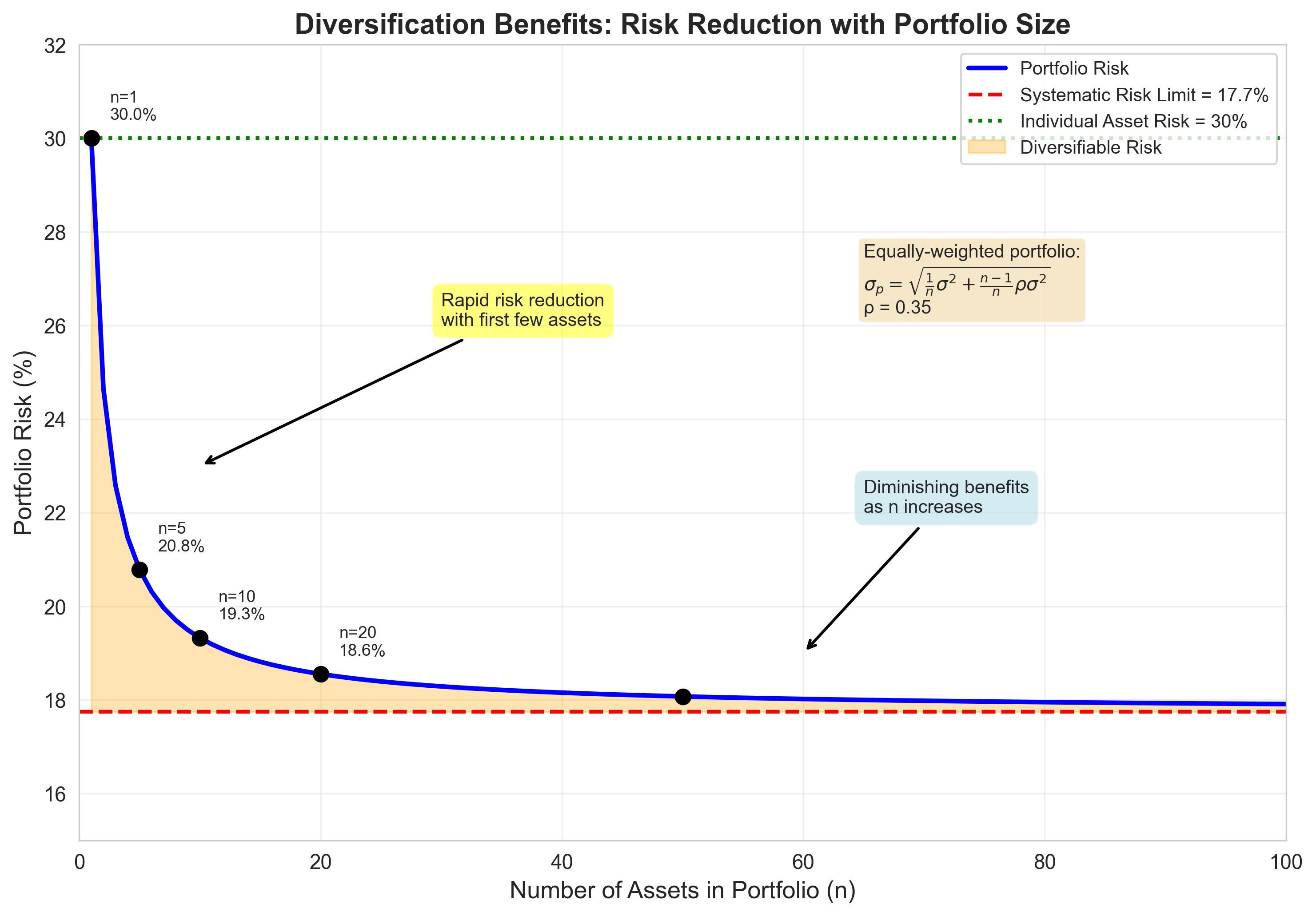
Figure: Portfolio risk decreases as the number of assets increases, but approaches a limit (systematic risk) that cannot be diversified away.
5. Three Risky Securities
With three risky assets:
- The weight space is two-dimensional
- The attainable set fills an area
Yet the efficient set collapses to a curve.
More choice does not mean more freedom.
Three-Asset Portfolio Space:
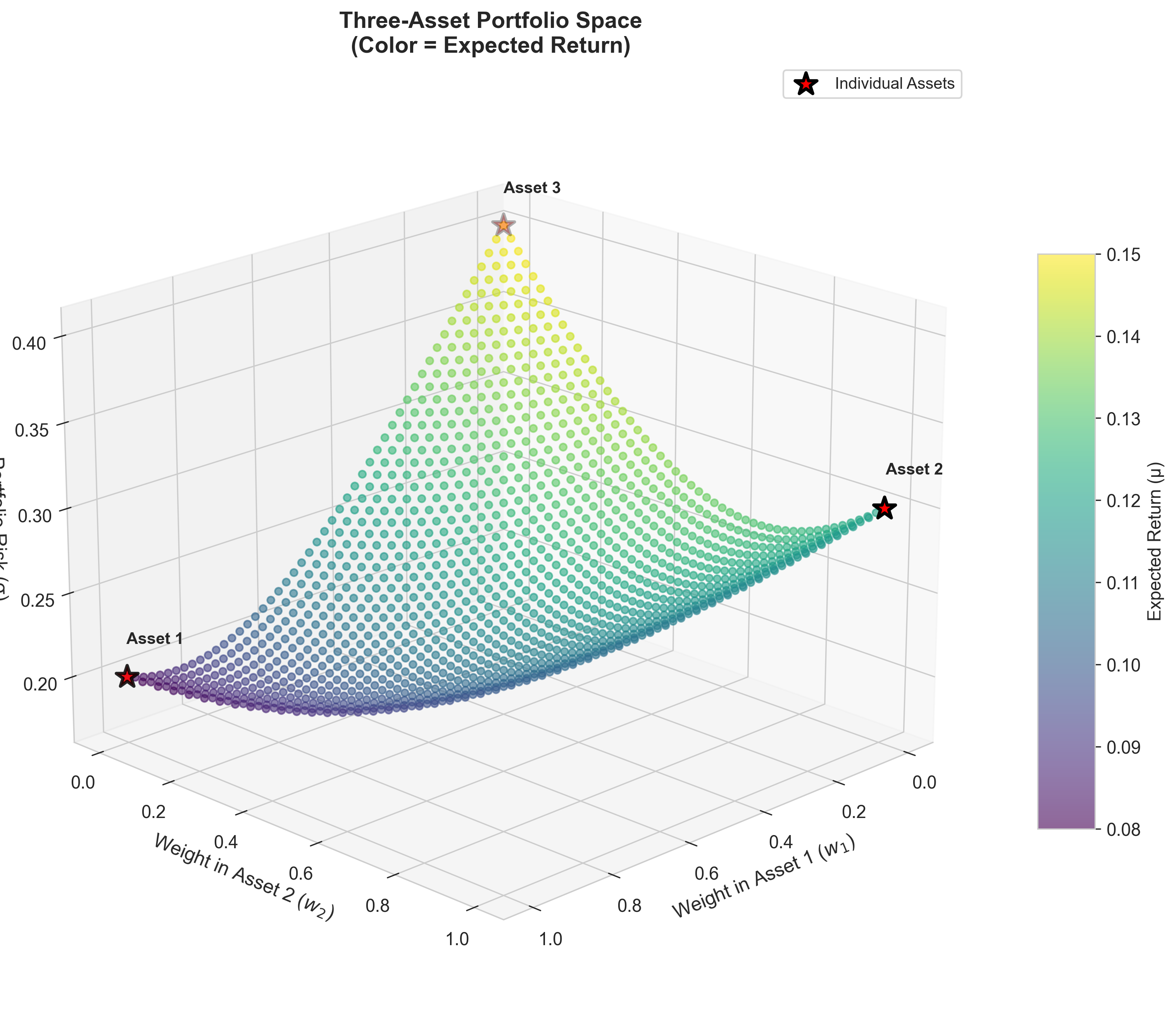
Figure: Portfolio possibilities in three-asset space. The simplex shows all valid portfolios where weights sum to 1. Color indicates expected return.
Return and Risk
For three assets:
\[ R_p = w_1R_1 + w_2R_2 + w_3R_3 \]
\[ \sigma_p^2 = w^\top \Sigma w \]
With \(w_1 + w_2 + w_3 = 1\).
Same equations. Higher dimension.
6. Minimum Variance Portfolio (MVP)
The minimum variance portfolio solves:
\[ \min_w \quad w^\top \Sigma w \]
subject to:
\[ u^\top w = 1 \]
Expected returns play no role here.
Risk comes first.
Why find the MVP?
- Anchors the efficient frontier
- Minimum risk achievable with given assets
- Starting point for efficient portfolios
Derivation via Lagrange Multipliers
Step 1: Form the Lagrangian
\[ \mathcal{L}(w,\lambda) = w^\top \Sigma w + \lambda(u^\top w - 1) \]
Where: * \(\lambda\) is the Lagrange multiplier * The constraint \(u^\top w = 1\) ensures weights sum to 1
Step 2: Take first-order conditions
Differentiate with respect to \(w\):
\[ \frac{\partial \mathcal{L}}{\partial w} = 2\Sigma w + \lambda u = 0 \]
Differentiate with respect to \(\lambda\):
\[ \frac{\partial \mathcal{L}}{\partial \lambda} = u^\top w - 1 = 0 \]
This is linear algebra, not magic.
Solving for MVP Weights
From the first condition:
\[ 2\Sigma w + \lambda u = 0 \]
Rearranging:
\[ \Sigma w = -\frac{\lambda}{2} u \]
Multiply both sides by \(\Sigma^{-1}\):
\[ w = -\frac{\lambda}{2} \Sigma^{-1} u \]
Apply the constraint \(u^\top w = 1\):
\[ u^\top w = -\frac{\lambda}{2} u^\top \Sigma^{-1} u = 1 \]
Solve for \(\lambda\):
\[ \lambda = -\frac{2}{u^\top \Sigma^{-1} u} \]
Substitute back:
\[ \boxed{w^{\text{MVP}} = \frac{\Sigma^{-1}u}{u^\top \Sigma^{-1}u}} \]
This formula appears everywhere for a reason.
Properties of the MVP
Weights sum to one (by construction)
Unique (if \(\Sigma\) is invertible)
Does not depend on expected returns
- Pure risk minimization
- No assumptions about investor preferences
Computationally stable (usually)
- Depends only on covariance matrix
- Less sensitive to estimation error than mean-variance portfolios
Numerical Example: Three-Asset MVP
Using our previous covariance matrix:
\[ \Sigma = \begin{pmatrix} 0.04 & 0.01 & 0.02 \\ 0.01 & 0.09 & 0.03 \\ 0.02 & 0.03 & 0.16 \end{pmatrix} \]
First compute \(\Sigma^{-1}\):
\[ \Sigma^{-1} \approx \begin{pmatrix} 28.09 & -2.25 & -2.81 \\ -2.25 & 12.36 & -0.56 \\ -2.81 & -0.56 & 7.30 \end{pmatrix} \]
Then:
\[ \Sigma^{-1}u = \begin{pmatrix} 23.03 \\ 9.55 \\ 3.93 \end{pmatrix}, \quad u^\top \Sigma^{-1}u = 36.51 \]
MVP weights:
\[ w^{\text{MVP}} = \begin{pmatrix} 0.631 \\ 0.262 \\ 0.108 \end{pmatrix} \]
Portfolio variance: \(\sigma_{\text{MVP}}^2 = 0.0274\), so \(\sigma_{\text{MVP}} = 16.55\%\)
Interpretation: Most weight in Asset 1 (lowest variance), least in Asset 3 (highest variance).
7. Minimum Variance Set and Line
As we vary expected return constraints:
\[ w^\top \mu = \mu_p \]
we obtain a family of portfolios.
Their image in \((\sigma, \mu)\) space forms the minimum variance frontier.
This is the set of all portfolios with minimum variance for each target return.
Optimization Problem for Target Return
For a target expected return \(\mu_p\), solve:
\[ \min_w \quad w^\top \Sigma w \]
subject to:
\[ u^\top w = 1, \quad w^\top \mu = \mu_p \]
Lagrangian:
\[ \mathcal{L}(w,\lambda_1,\lambda_2) = w^\top \Sigma w + \lambda_1(u^\top w - 1) + \lambda_2(w^\top \mu - \mu_p) \]
First-order condition:
\[ 2\Sigma w + \lambda_1 u + \lambda_2 \mu = 0 \]
Solving this system yields the entire efficient frontier.
General Solution
The solution has the form:
\[ w^*(\mu_p) = w^{\text{MVP}} + \lambda(\mu_p) \cdot w^{\text{diff}} \]
Where: * \(w^{\text{MVP}}\) is the minimum variance portfolio * \(w^{\text{diff}}\) is a portfolio orthogonal to the MVP * \(\lambda(\mu_p)\) scales based on target return
Key insight: All efficient portfolios are combinations of two “basis” portfolios.
This is the two-fund theorem for risky assets.
Minimum Variance Line
Without a risk-free asset:
- The efficient set is a curve (hyperbola in \((\sigma^2, \mu)\) space)
- Only the upper branch is relevant (above the MVP)
- Below the MVP, portfolios are dominated
Efficiency is selective.
Graphical representation:
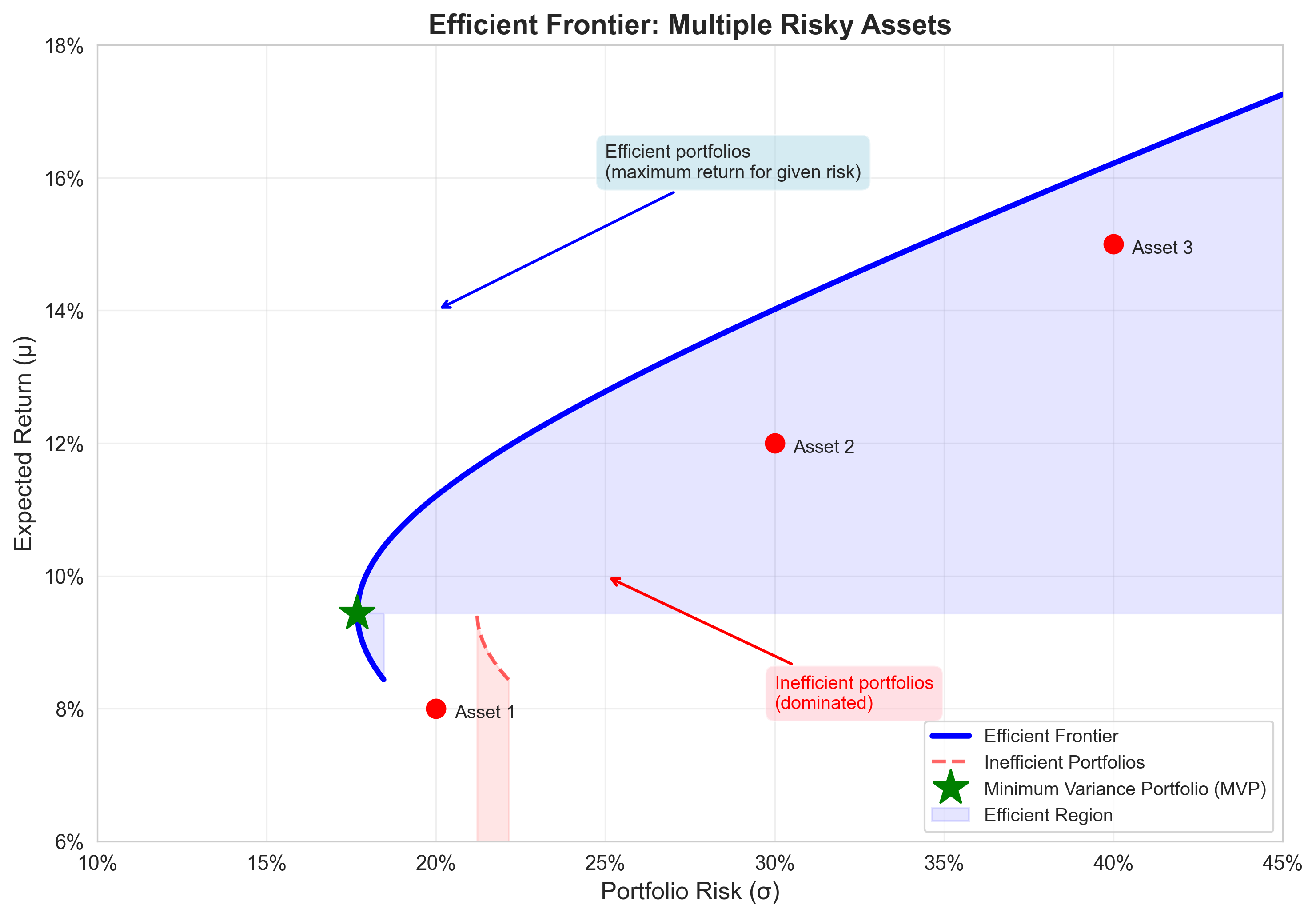
Figure: The efficient frontier shows the minimum risk for each level of return. Only the upper branch (above MVP) is efficient.
- The MVP is the leftmost point
- Moving up the frontier increases both return and risk
- The lower branch is inefficient (higher risk for same return)
8. Adding the Risk-Free Asset
Once a risk-free asset is available:
- The efficient frontier becomes a straight line
- Only one risky portfolio matters
This line dominates all others.
Geometry collapses again.
Capital Allocation Line with Tangency Portfolio:
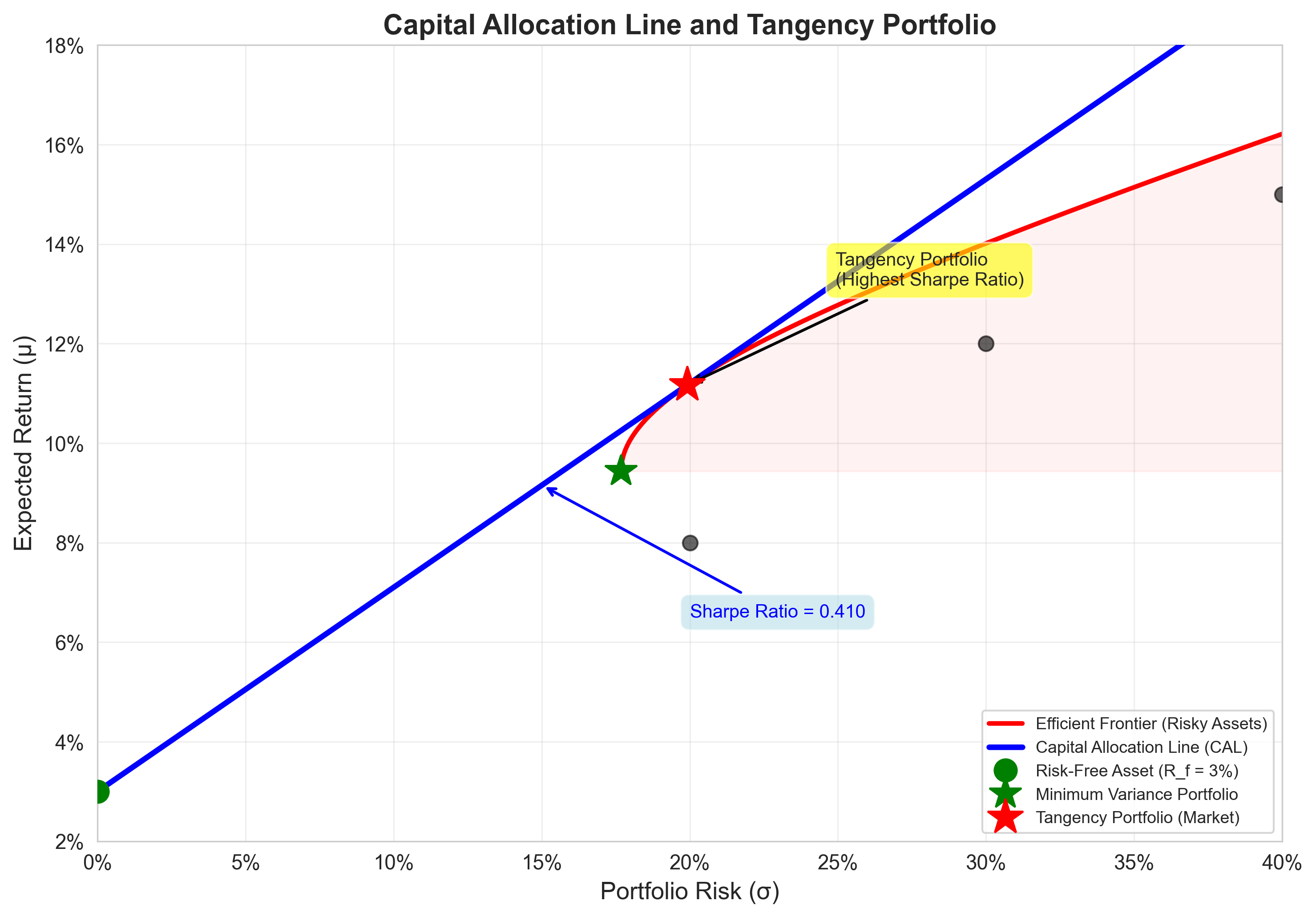
Figure: The CAL (blue line) is tangent to the efficient frontier at the tangency portfolio. This portfolio has the highest Sharpe ratio among all risky portfolios.
Capital Allocation Line (CAL) - Revisited
With \(n\) risky assets and a risk-free asset:
- Combine the risk-free asset with any risky portfolio
- The best combination uses the tangency portfolio or market portfolio
The CAL equation:
\[ \mu_p = R_f + \frac{\mu_M - R_f}{\sigma_M} \sigma_p \]
Where \(M\) is the market portfolio (the tangency portfolio).
Key result: The Capital Allocation Line dominates all other portfolios in the risky asset space.
Every investor should hold: 1. The market portfolio (risky assets) 2. The risk-free asset
Only the proportions differ based on risk preferences.
9. Market Portfolio
The market portfolio is:
- The tangency portfolio
- The risky portfolio with the highest Sharpe ratio
- The portfolio all investors hold (in equilibrium)
It solves:
\[ \max_w \quad \frac{w^\top \mu - R_f}{\sqrt{w^\top \Sigma w}} \]
subject to:
\[ u^\top w = 1 \]
This is the Sharpe ratio maximization problem.
Derivation of Market Portfolio
Equivalently, we can solve the Sharpe ratio maximization directly:
\[ \max_w \quad \frac{w^\top \mu - R_f}{\sqrt{w^\top \Sigma w}} \]
subject to:
\[ u^\top w = 1 \]
Lagrangian:
\[ \mathcal{L} = \frac{w^\top \mu - R_f}{\sqrt{w^\top \Sigma w}} + \lambda(u^\top w - 1) \]
First-order condition:
\[ \frac{1}{\sqrt{w^\top \Sigma w}}[\mu - \frac{(w^\top \mu - R_f)}{w^\top \Sigma w}\Sigma w] + \lambda u = 0 \]
Simplifying and rearranging (with too much effort):
\[ \Sigma w \propto \mu - R_f u \]
With the budget constraint applied, this yields:
\[ w^{\text{M}} = \frac{\Sigma^{-1}(\mu - R_fu)}{u^\top \Sigma^{-1}(\mu - R_fu)} \]
Characterization of the Market Portfolio
After applying constraints and simplifying:
\[ w^{\text{M}} \propto \Sigma^{-1}(\mu - R_fu) \]
With normalization:
\[ w^{\text{M}} = \frac{\Sigma^{-1}(\mu - R_fu)}{u^\top \Sigma^{-1}(\mu - R_fu)} \]
Key observations:
- Depends on \(\mu - R_f\) (excess returns)
- Inversely weighted by covariance matrix
- Does not depend on risk aversion
Interpretation
- Everyone holds the same risky portfolio (the market portfolio)
- Differences arise only through leverage (borrowing/lending at \(R_f\))
- Risk-averse investors hold more of the risk-free asset
- Risk-tolerant investors borrow and lever up the market portfolio
Numerical Example: Market Portfolio
Using our three-asset example with:
\[ \mu = \begin{pmatrix} 0.08 \\ 0.12 \\ 0.15 \end{pmatrix}, \quad R_f = 0.03 \]
\[ \Sigma^{-1} \approx \begin{pmatrix} 28.09 & -2.25 & -2.81 \\ -2.25 & 12.36 & -0.56 \\ -2.81 & -0.56 & 7.30 \end{pmatrix} \]
Compute \(\mu - R_fu\):
\[ \mu - R_fu = \begin{pmatrix} 0.05 \\ 0.09 \\ 0.12 \end{pmatrix} \]
Then:
\[ \Sigma^{-1}(\mu - R_fu) = \begin{pmatrix} 0.768 \\ 0.984 \\ 0.689 \end{pmatrix} \]
Sum: \(0.768 + 0.984 + 0.689 = 2.441\)
Market portfolio weights:
\[ w^{\text{M}} = \begin{pmatrix} 0.315 \\ 0.403 \\ 0.282 \end{pmatrix} \]
Expected return: \(\mu_M = 0.315(0.08) + 0.403(0.12) + 0.282(0.15) = 11.4\%\)
Variance: \(\sigma_M^2 = 0.0332\), so \(\sigma_M = 18.2\%\)
Sharpe ratio: \(\frac{0.114 - 0.03}{0.182} = 0.462\)
10. Exercises
Exercise 1: Computing the MVP
Given three assets with expected returns and covariance matrix:
\[ \mu = \begin{pmatrix} 0.07 \\ 0.10 \\ 0.13 \end{pmatrix}, \quad \Sigma = \begin{pmatrix} 0.09 & 0.02 & 0.01 \\ 0.02 & 0.16 & 0.03 \\ 0.01 & 0.03 & 0.25 \end{pmatrix} \]
Tasks: 1. Compute the minimum variance portfolio weights 2. Calculate the expected return and standard deviation of the MVP 3. Verify that the weights sum to one 4. Interpret the result: which asset gets the most weight and why?
Exercise 2: Efficient Frontier
Using the same three assets from Exercise 1:
Tasks: 1. Find the portfolio with target expected return \(\mu_p = 10\%\) 2. Calculate the variance of this portfolio 3. Compare its risk to the MVP 4. Is this portfolio on the efficient frontier? Explain.
Hint: Set up the Lagrangian with two constraints and solve the first-order conditions.
Exercise 3: Market Portfolio
Given \(R_f = 0.04\) and the data from Exercise 1:
Tasks: 1. Compute the market portfolio (tangency portfolio) 2. Calculate its expected return, variance, and Sharpe ratio 3. Compare the market portfolio to the MVP: which has higher expected return? Which has lower risk? 4. Explain why the market portfolio does not depend on individual risk aversion
Exercise 4: Diversification Analysis
Consider \(n\) identical assets, each with: * Expected return: \(\mu = 12\%\) * Variance: \(\sigma^2 = 0.16\) * Pairwise correlation: \(\rho = 0.3\)
Tasks: 1. Write the formula for the variance of an equally-weighted portfolio 2. Compute portfolio variance for \(n = 2, 5, 10, 50, 100\) 3. What is the limiting variance as \(n \to \infty\)? 4. What percentage of risk is diversifiable? What percentage is systematic?
Hint: Use \(\sigma_p^2 = \frac{1}{n}\sigma^2 + \frac{n-1}{n}\rho\sigma^2\)
Exercise 5: Constrained Optimization
Prove that the MVP weights sum to one using the formula:
\[ w^{\text{MVP}} = \frac{\Sigma^{-1}u}{u^\top \Sigma^{-1}u} \]
Steps: 1. Take the sum of weights: \(\sum_{i=1}^n w_i = u^\top w^{\text{MVP}}\) 2. Substitute the MVP formula 3. Simplify to show the result equals 1
Explain why this property is economically necessary (budget constraint).
Final Takeaways
- Multi-asset portfolios require linear algebra
- Portfolio return: \(\mu_p = w^\top \mu\) (linear)
- Portfolio variance: \(\sigma_p^2 = w^\top \Sigma w\) (quadratic)
- Optimization uses Lagrange multipliers
- Diversification has limits
- Can eliminate idiosyncratic risk
- Cannot eliminate systematic (correlated) risk
- Benefits diminish as \(n\) increases
- The MVP anchors the efficient frontier
- Minimum achievable risk with given assets
- Does not depend on expected returns
- Computationally more stable than mean-variance portfolios
- The efficient frontier is a curve (without risk-free
asset)
- Hyperbola in \((\sigma^2, \mu)\) space
- Only upper branch is efficient
- All efficient portfolios are linear combinations of two basis portfolios
- Adding a risk-free asset collapses the frontier to a
line
- The Capital Allocation Line (CAL)
- Slope = Sharpe ratio of tangency portfolio
- All investors hold the same risky portfolio (two-fund separation)
- The market portfolio emerges naturally
- Tangency portfolio = market portfolio (in equilibrium)
- Maximizes Sharpe ratio
- Does not depend on risk aversion
- Foundation for CAPM
Next lecture: We will turn these portfolio results into asset pricing theory via the Capital Asset Pricing Model (CAPM).