Capital Asset Pricing Model
(CAPM)
Sukrit Mittal Franklin Templeton Investments
Outline
- Why CAPM?
- Assumptions and market setting
- From portfolio choice to equilibrium
- Derivation of CAPM
- Security Market Line (SML)
- Systematic vs idiosyncratic risk
- Characteristic line
- Empirical interpretation and limits
- Exercises
1. Why CAPM?
Up to now we solved investor problems.
- How should I allocate my wealth?
- What is the optimal portfolio given my risk preferences?
CAPM answers a different question:
How are assets priced in equilibrium?
This is not about optimal portfolios.
It is about consistency across the entire market.
The fundamental question: If all investors are
mean-variance optimizers, what must expected returns look like?
What CAPM Is—and Is Not
CAPM is: A model of how risk translates into return
CAPM is not: A trading strategy
It is a benchmark.
Historical Context
Developed independently by:
- William Sharpe (1964)
- John Lintner (1965)
- Jan Mossin (1966)
Sharpe won the Nobel Prize in Economics (1990) for this work.
The model revolutionized finance by providing a testable theory of
expected returns.
2. Market Setting and
Assumptions
We assume:
Mean–variance optimization: All investors choose
portfolios based only on expected return and variance
Homogeneous expectations: All investors agree
on:
- Expected returns \(\mu\)
- Covariance matrix \(\Sigma\)
- Risk-free rate \(R_f\)
Perfect capital markets:
- No transaction costs
- No taxes
- Assets are infinitely divisible
- All assets are marketable and liquid
Single-period horizon: All investors have the
same investment horizon
Risk-free borrowing and lending: Investors can
lend or borrow unlimited amounts at rate \(R_f\)
These assumptions are strong.
Why These Assumptions?
What each assumption enables:
- Mean-variance: Reduces preferences to two
dimensions
- Homogeneous expectations: Ensures all investors
face same optimization problem
- Perfect markets: Eliminates frictions that
complicate pricing
- Single period: Avoids dynamic complexities
- Risk-free rate: Creates separation between risk and
return
Relaxing these assumptions leads to extensions and alternative
models.
But understanding CAPM requires accepting them first.
Critique of Assumptions
Homogeneous expectations is the most
controversial:
- Investors clearly disagree about future returns
- Disagreement is the reason trading occurs
- Yet: if disagreements are “rational,” maybe they average out in
equilibrium
Perfect markets:
- Transaction costs exist but are small for large investors
- Taxes matter but CAPM can be extended to incorporate them
- The model still provides useful baseline predictions
The question is not whether assumptions are true.
The question is whether the model is useful despite them.
3. From Portfolio Choice
to Equilibrium
From Lecture 07, we know:
- All mean-variance investors (with same expectations) hold the same
risky portfolio
- This portfolio is the tangency portfolio (maximizes
Sharpe ratio)
- Differences arise only via leverage (mix with risk-free asset)
In equilibrium:
The risky portfolio held by everyone must be the market
portfolio.
Why? Market clearing.
- If everyone wants to hold portfolio \(P\)
- But some asset \(i\) is not in
\(P\) (or has wrong weight)
- Then there is excess supply or demand for asset \(i\)
- Prices must adjust until \(P\)
equals the market portfolio
This is the critical step.
The Market Portfolio
The market portfolio \(M\) contains:
- All risky assets
- In proportion to their market values
Definition:
\[
w_i^M = \frac{\text{Market value of asset } i}{\text{Total market value
of all assets}}
\]
Examples:
- If a stock has market cap 100B USD and total market is 10T USD, then
\(w_i = 0.01\)
- The S&P 500 (value-weighted) approximates the U.S. equity market
portfolio
- A global market portfolio includes all stocks, bonds, real estate,
etc.
No asset can escape the market.
If it exists, it is priced.
Equilibrium Condition
In equilibrium, two conditions must hold:
Optimality: Each investor holds an optimal
portfolio given prices
Market clearing: Total demand = Total supply for
every asset
Combining these:
\[
\text{Aggregate holdings} = \text{Market portfolio}
\]
Since everyone holds the tangency portfolio, it must equal the market
portfolio.
This pins down expected returns.
4. Risk Decomposition
Consider an asset \(i\) with return
\(R_i\).
Decompose its risk relative to the market \(R_M\).
Only part of this risk matters, rest is diversifiable noise.
Total Risk Decomposition
Any asset’s return can be written as:
\[
R_i = \mathbb{E}[R_i] + \beta_i(R_M - \mathbb{E}[R_M]) + \varepsilon_i
\]
Where: * \(\beta_i(R_M -
\mathbb{E}[R_M])\) = systematic component (market-driven) * \(\varepsilon_i\) = idiosyncratic component
(asset-specific) * \(\mathbb{E}[\varepsilon_i]
= 0\) and \(\text{Cov}(\varepsilon_i,
R_M) = 0\) (by construction)
Total variance:
\[
\text{Var}(R_i) = \beta_i^2 \text{Var}(R_M) + \text{Var}(\varepsilon_i)
\]
- First term: systematic risk (cannot diversify
away)
- Second term: idiosyncratic risk (diversifies away
in large portfolios)
Beta: Measuring Systematic
Risk
Define beta:
\[
\beta_i = \frac{\text{Cov}(R_i, R_M)}{\text{Var}(R_M)}
\]
Beta measures:
Sensitivity to market movements.
Interpretation:
- \(\beta_i = 1\): Asset moves
one-for-one with the market
- \(\beta_i > 1\): Asset is more
volatile than the market (aggressive)
- \(\beta_i < 1\): Asset is less
volatile than the market (defensive)
- \(\beta_i = 0\): Asset is
uncorrelated with the market
- \(\beta_i < 0\): Asset moves
opposite to the market (rare, e.g., gold)
This is the only risk investors are paid for.
Why? Because idiosyncratic risk can be diversified away.
5. Derivation of CAPM
Consider the market portfolio \(M\).
For any asset \(i\):
- Adding \(i\) to \(M\) must not improve the Sharpe ratio
Otherwise, \(M\) would not be
optimal.
This restriction pins down expected returns.
Derivation via
Marginal Contribution to Risk
Consider a portfolio with weight \(\alpha\) in asset \(i\) and \((1-\alpha)\) in the market portfolio \(M\).
Portfolio return:
\[
R_p(\alpha) = \alpha R_i + (1-\alpha) R_M
\]
Portfolio variance:
\[
\sigma_p^2(\alpha) = \alpha^2 \sigma_i^2 + (1-\alpha)^2 \sigma_M^2 +
2\alpha(1-\alpha) \text{Cov}(R_i, R_M)
\]
At \(\alpha = 0\) (pure market
portfolio), the Sharpe ratio must be maximized.
First-order condition for maximum Sharpe ratio:
\[
\frac{d}{d\alpha}\left[\frac{\mathbb{E}[R_p(\alpha)] -
R_f}{\sigma_p(\alpha)}\right]\Bigg|_{\alpha=0} = 0
\]
Derivation (continued)
The Sharpe ratio of the mixed portfolio is:
\[
S(\alpha) = \frac{\mathbb{E}[R_p(\alpha)] - R_f}{\sigma_p(\alpha)}
\]
For \(M\) to be optimal, the
derivative with respect to \(\alpha\)
must be zero at \(\alpha = 0\).
Step 1: Derivative of expected return
\[
\frac{d\mathbb{E}[R_p]}{d\alpha} = \mathbb{E}[R_i] - \mathbb{E}[R_M]
\]
Step 2: Derivative of variance
\[
\frac{d\sigma_p^2}{d\alpha} = 2\alpha \sigma_i^2 +
2(1-2\alpha)\sigma_M^2 - 2(1-2\alpha)\text{Cov}(R_i, R_M)\]
At \(\alpha = 0\):
\[
\frac{d\sigma_p^2}{d\alpha}\Bigg|_{\alpha=0} = 2[\text{Cov}(R_i, R_M) -
\sigma_M^2]
\]
Step 3: Derivative of standard deviation
\[
\frac{d\sigma_p}{d\alpha}\Bigg|_{\alpha=0} =
\frac{1}{\sigma_M}[\text{Cov}(R_i, R_M) - \sigma_M^2]
\]
Step 4: Apply quotient rule to Sharpe ratio
\[
\frac{dS}{d\alpha} = \frac{\frac{d\mathbb{E}[R_p]}{d\alpha} \cdot
\sigma_p - (\mathbb{E}[R_p] - R_f) \cdot
\frac{d\sigma_p}{d\alpha}}{\sigma_p^2}
\]
At \(\alpha = 0\), set numerator to
zero:
\[
[\mathbb{E}[R_i] - \mathbb{E}[R_M]] \sigma_M = [\mathbb{E}[R_M] - R_f]
\cdot \frac{\text{Cov}(R_i, R_M) - \sigma_M^2}{\sigma_M}
\]
Step 5: Simplify
CAPM Equation
Rearranging:
\[
\mathbb{E}[R_i] - \mathbb{E}[R_M] = \frac{\mathbb{E}[R_M] -
R_f}{\sigma_M^2}[\text{Cov}(R_i, R_M) - \sigma_M^2]
\]
For the market portfolio itself, \(\text{Cov}(R_M, R_M) = \sigma_M^2\), so
this holds with equality.
For any other asset \(i\):
\[
\mathbb{E}[R_i] = \mathbb{E}[R_M] + \frac{\mathbb{E}[R_M] -
R_f}{\sigma_M^2}[\text{Cov}(R_i, R_M) - \sigma_M^2]
\]
Rearranging:
\[
\mathbb{E}[R_i] = R_f + \frac{\text{Cov}(R_i,
R_M)}{\sigma_M^2}[\mathbb{E}[R_M] - R_f]
\]
Using \(\beta_i = \frac{\text{Cov}(R_i,
R_M)}{\sigma_M^2}\):
\[
\boxed{\mathbb{E}[R_i] - R_f = \beta_i\big( \mathbb{E}[R_M] - R_f \big)}
\]
This is the CAPM equation.
6. Security Market Line (SML)
Plot expected return against beta.
The CAPM predicts a straight line:
\[
\mathbb{E}[R_i] = R_f + \beta_i (\mathbb{E}[R_M] - R_f)
\]
This line is the Security Market Line (SML).
Key points on the SML:
- Risk-free asset: \(\beta
= 0\), \(\mathbb{E}[R] =
R_f\)
- Market portfolio: \(\beta
= 1\), \(\mathbb{E}[R] =
\mathbb{E}[R_M]\)
- Aggressive asset: \(\beta
> 1\), \(\mathbb{E}[R] >
\mathbb{E}[R_M]\)
- Defensive asset: \(0 <
\beta < 1\), \(R_f <
\mathbb{E}[R] < \mathbb{E}[R_M]\)
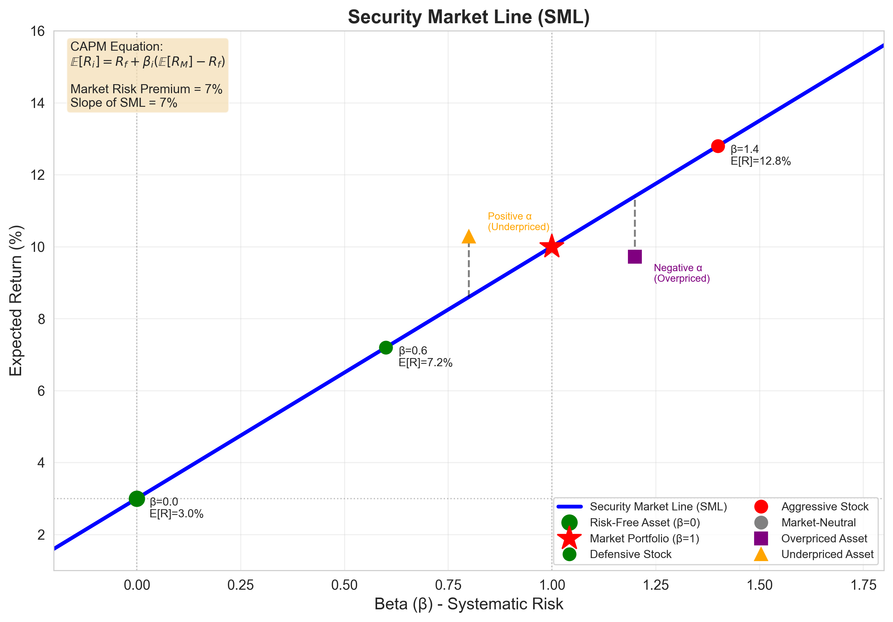
Graphical Representation:
Figure: The Security Market Line shows the linear relationship
between beta and expected return predicted by CAPM. Assets above the
line are underpriced (positive alpha), while those below are overpriced
(negative alpha).
Interpretation of the SML
Components:
- Intercept: \(R_f\)
(risk-free rate)
- Slope: \(\mathbb{E}[R_M]
- R_f\) (market risk premium)
Economic interpretation:
\[
\text{Expected excess return} = \beta \times \text{Market risk premium}
\]
- You earn the risk-free rate for waiting
- You earn a premium proportional to systematic risk
(\(\beta\))
- Idiosyncratic risk earns no premium (it can be diversified)
Asset pricing implications:
- Assets above the line: underpriced (higher return
than CAPM predicts)
- Assets on the line: fairly priced
- Assets below the line: overpriced (lower return
than CAPM predicts)
In theory.
Numerical Example: Using the
SML
Suppose: * \(R_f = 3\%\) * \(\mathbb{E}[R_M] = 10\%\) * Market risk
premium: \(\mathbb{E}[R_M] - R_f =
7\%\)
Asset A: \(\beta_A =
0.8\) (defensive)
\[
\mathbb{E}[R_A] = 0.03 + 0.8(0.10 - 0.03) = 0.03 + 0.056 = 8.6\%
\]
Asset B: \(\beta_B =
1.5\) (aggressive)
\[
\mathbb{E}[R_B] = 0.03 + 1.5(0.10 - 0.03) = 0.03 + 0.105 = 13.5\%
\]
Asset C: \(\beta_C =
1.2\), observed return = \(15\%\)
CAPM prediction:
\[
\mathbb{E}[R_C] = 0.03 + 1.2(0.07) = 11.4\%
\]
Actual return (15%) > CAPM prediction (11.4%)
Interpretation: Asset C is underpriced or has
positive alpha.
7. Systematic vs Idiosyncratic
Risk
Total risk decomposes into:
- Systematic risk (market-related,
undiversifiable)
- Idiosyncratic risk (asset-specific,
diversifiable)
Diversification eliminates only the latter.
Markets pay only for what cannot be diversified.
Mathematical Decomposition
Recall the risk decomposition:
\[
R_i = \mathbb{E}[R_i] + \beta_i(R_M - \mathbb{E}[R_M]) + \varepsilon_i
\]
Taking variance:
\[
\text{Var}(R_i) = \beta_i^2 \text{Var}(R_M) + \text{Var}(\varepsilon_i)
\]
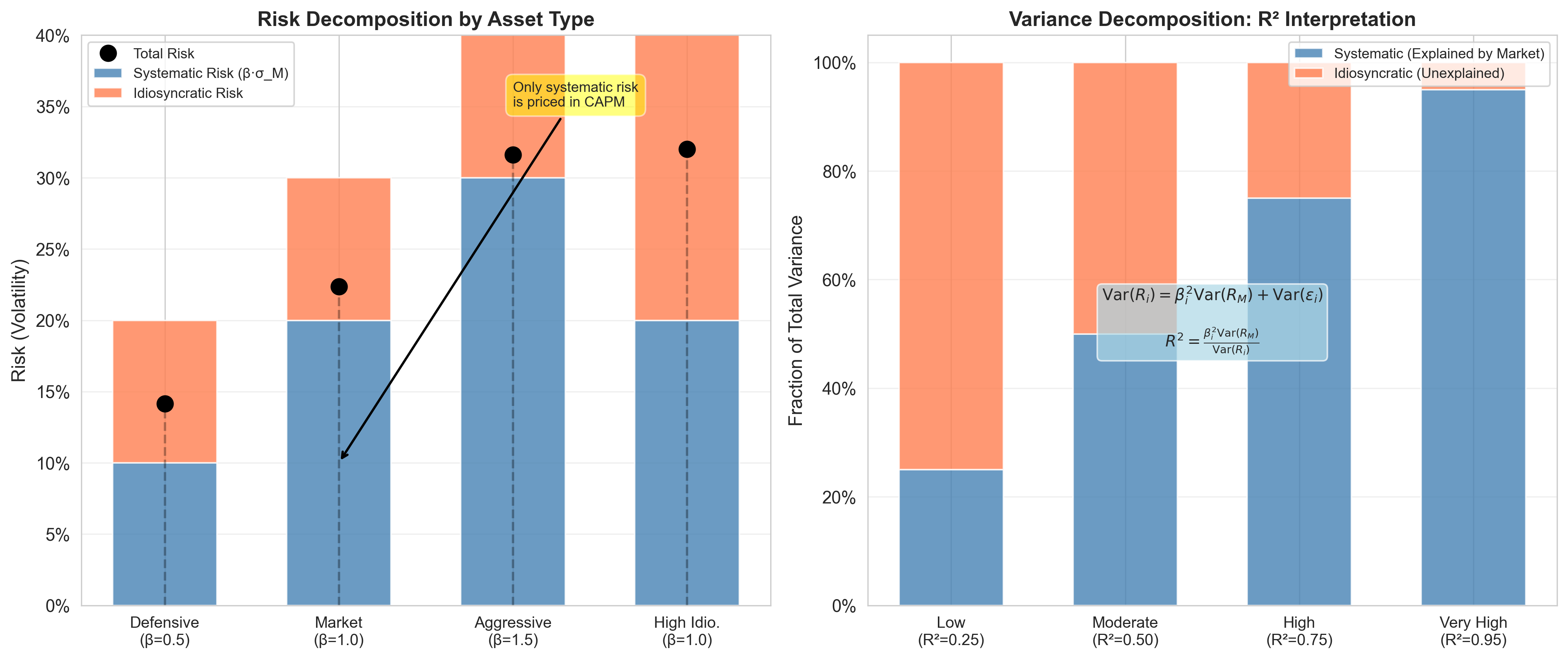
R-squared: Fraction of variance explained by the
market:
\[
R^2 = \frac{\beta_i^2 \text{Var}(R_M)}{\text{Var}(R_i)}
\]
- \(R^2 = 1\): All risk is systematic
(perfectly correlated with market)
- \(R^2 = 0\): All risk is
idiosyncratic (uncorrelated with market)
- Typical stock: \(R^2 \approx 0.3\)
(30% of variance is systematic)
Why Only Systematic Risk Is
Priced
Key insight: In a well-diversified portfolio,
idiosyncratic risks cancel out.
For a portfolio of \(n\) assets with
equal weights:
\[
R_p = \frac{1}{n}\sum_{i=1}^n R_i = \mathbb{E}[R_p] + \beta_p(R_M -
\mathbb{E}[R_M]) + \frac{1}{n}\sum_{i=1}^n \varepsilon_i
\]
Where \(\beta_p = \frac{1}{n}\sum_{i=1}^n
\beta_i\).
Variance of idiosyncratic component:
If \(\varepsilon_i\) are
uncorrelated with average variance \(\bar{\sigma}_\varepsilon^2\):
\[
\text{Var}\left(\frac{1}{n}\sum_{i=1}^n \varepsilon_i\right) =
\frac{\bar{\sigma}_\varepsilon^2}{n} \to 0 \text{ as } n \to \infty
\]
Conclusion: Large portfolios eliminate idiosyncratic
risk.
Since investors can diversify at zero cost, they won’t pay a premium
for bearing idiosyncratic risk.
Visual Decomposition:
Figure: (Left) Risk decomposition for different asset types
showing systematic and idiosyncratic components. (Right) R²
interpretation showing the fraction of variance explained by the
market.
Numerical Example:
Diversification
Consider 50 stocks, each with: * Beta: \(\beta_i = 1.2\) * Idiosyncratic variance:
\(\text{Var}(\varepsilon_i) = 0.04\) *
Market variance: \(\sigma_M^2 =
0.04\)
Individual stock variance:
\[
\text{Var}(R_i) = (1.2)^2(0.04) + 0.04 = 0.0576 + 0.04 = 0.0976
\]
Standard deviation: \(\sigma_i =
31.2\%\)
Equally-weighted portfolio variance:
\[
\text{Var}(R_p) = (1.2)^2(0.04) + \frac{0.04}{50} = 0.0576 + 0.0008 =
0.0584
\]
Standard deviation: \(\sigma_p =
24.2\%\)
Risk reduction: From 31.2% to 24.2% (22%
reduction)
- Systematic risk: \(\sqrt{0.0576} =
24\%\) (unchanged)
- Idiosyncratic risk: nearly eliminated
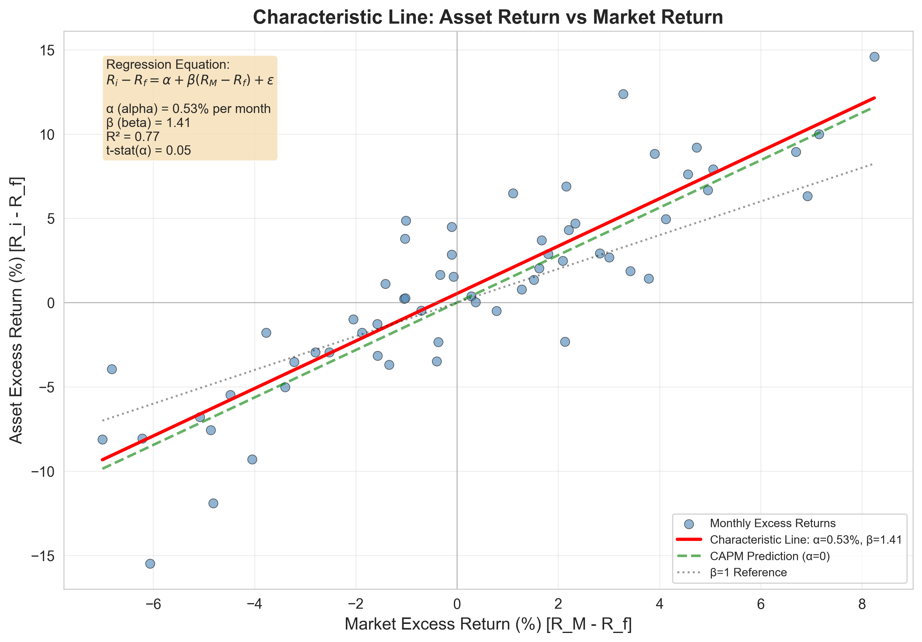
8. Characteristic Line
The characteristic line relates an asset’s excess
return to the market’s excess return:
\[
R_i - R_f = \alpha_i + \beta_i (R_M - R_f) + \varepsilon_i
\]
This is a regression equation.
Components:
- \(\alpha_i\) =
alpha (intercept) = abnormal return
- \(\beta_i\) = beta
(slope) = systematic risk exposure
- \(\varepsilon_i\) = residual
(idiosyncratic component)
Assumptions:
- \(\mathbb{E}[\varepsilon_i] =
0\)
- \(\text{Cov}(\varepsilon_i, R_M) =
0\)
Graphical Representation:
Figure: The characteristic line shows the regression of asset
excess returns against market excess returns. The slope is beta, and the
intercept is alpha. Positive alpha indicates outperformance relative to
CAPM predictions.
Interpretation of Parameters
Beta (\(\beta_i\)):
- Measures systematic exposure to market risk
- \(\beta_i = \frac{\text{Cov}(R_i - R_f,
R_M - R_f)}{\text{Var}(R_M - R_f)}\)
- Estimated as the slope in time-series regression
Alpha (\(\alpha_i\)):
- Measures abnormal return (above or below CAPM
prediction)
- In CAPM equilibrium: \(\alpha_i =
0\) for all assets
- Nonzero alpha suggests:
- Mispricing
- Model misspecification
- Superior skill (if persistent)
Residual (\(\varepsilon_i\)):
- Idiosyncratic noise
- Diversifies away in portfolios
- Variance \(\text{Var}(\varepsilon_i)\) measures
idiosyncratic risk
In CAPM:
\[
\alpha_i = 0
\]
Nonzero alpha is a claim.
Extraordinary claims require extraordinary evidence.
Estimating Beta:
Time-Series Regression
Data: Historical returns for asset \(i\) and market \(M\) over \(T\) periods
Regression:
\[
r_{i,t} - r_{f,t} = \alpha_i + \beta_i(r_{M,t} - r_{f,t}) +
\varepsilon_{i,t}
\]
for \(t = 1, 2, \ldots, T\)
Ordinary Least Squares (OLS) estimate:
\[
\hat{\beta}_i = \frac{\sum_{t=1}^T (r_{i,t} - \bar{r}_i)(r_{M,t} -
\bar{r}_M)}{\sum_{t=1}^T (r_{M,t} - \bar{r}_M)^2}
\]
Standard error:
\[
\text{SE}(\hat{\beta}_i) =
\frac{\hat{\sigma}_\varepsilon}{\sqrt{\sum_{t=1}^T (r_{M,t} -
\bar{r}_M)^2}}
\]
Where \(\hat{\sigma}_\varepsilon\)
is the standard deviation of residuals.
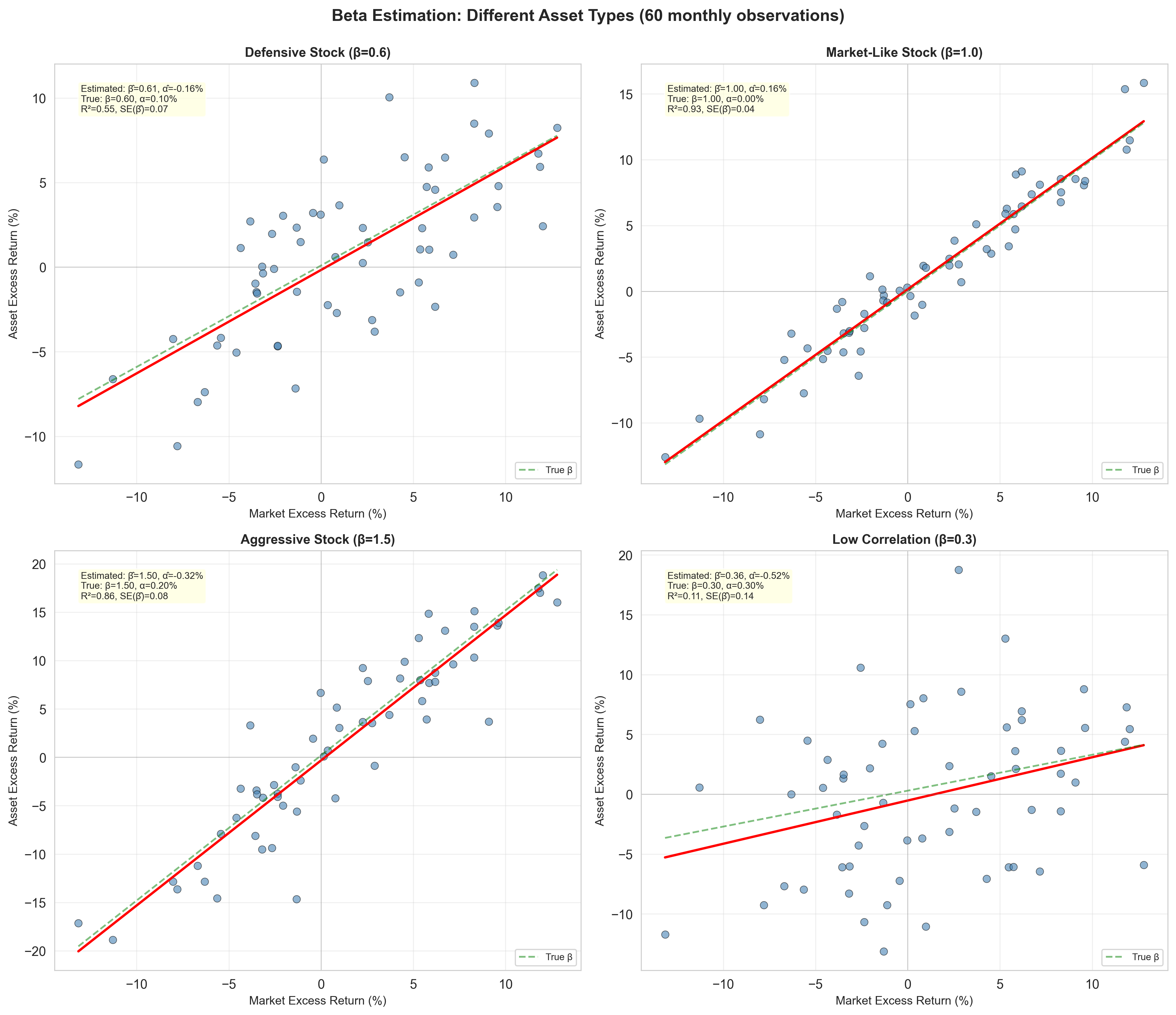
Beta Estimation Examples:
Figure: Beta estimation for different asset types using
time-series regression. Each panel shows 60 monthly observations with
the fitted characteristic line. Note how R² varies with the strength of
market correlation.
Numerical Example: Estimating
Beta
Suppose we have 60 monthly returns for Stock XYZ and the S&P
500.
Regression results:
\[
r_{\text{XYZ},t} - r_{f,t} = 0.005 + 1.35(r_{M,t} - r_{f,t}) +
\varepsilon_t
\]
- \(\hat{\alpha} = 0.005\) (0.5% per
month = 6% per year)
- \(\hat{\beta} = 1.35\) (more
volatile than market)
- \(t\)-statistic for \(\alpha\): \(t =
2.1\) (marginally significant)
- \(R^2 = 0.42\) (42% of variance
explained by market)
Interpretation:
- XYZ is an aggressive stock (\(\beta >
1\))
- It appears to have positive alpha (outperforms CAPM prediction)
- But statistical significance is weak — could be luck
CAPM prediction: With \(R_f = 2\%\) and \(\mathbb{E}[R_M] = 9\%\):
\[
\mathbb{E}[R_{\text{XYZ}}] = 0.02 + 1.35(0.09 - 0.02) = 11.45\%
\]
If alpha persists, expected return would be: \(11.45\% + 6\% = 17.45\%\)
9. Empirical Reality
CAPM is elegant. Reality is less cooperative.
Empirically:
- Betas are unstable over time
- Many anomalies exist (size, value, momentum)
- Alpha is often statistically significant
But CAPM survives as a benchmark.
Empirical Tests of CAPM
Classic tests:
Black, Jensen, Scholes (1972): Found that
low-beta stocks earn higher returns than CAPM predicts
Roll’s critique (1977): CAPM is untestable
because the true market portfolio is unobservable
Key empirical findings:
- Flat Security Market Line: Empirically, the SML is
flatter than CAPM predicts
- Low-beta stocks earn more than predicted
- High-beta stocks earn less than predicted
- Anomalies:
- Size effect: Small stocks outperform large stocks
(controlling for beta)
- Value effect: High book-to-market stocks outperform
growth stocks
- Momentum: Past winners continue to outperform
- Time-varying betas: Beta estimates change with the
sample period
Why CAPM Fails Empirically
Violated assumptions:
- Not all investors are mean-variance optimizers
- Some use heuristics, others are constrained
- Heterogeneous expectations
- Investors disagree about expected returns
- Market frictions matter
- Transaction costs, taxes, short-sale constraints
- The market portfolio is unobservable
- S&P 500 ≠ true market portfolio
- Should include bonds, real estate, human capital, etc.
- Time-varying risk premiums
- Market risk premium changes with economic conditions
Despite failures, CAPM remains useful:
- Benchmark: Provides a null hypothesis for asset
pricing
- Risk adjustment: Beta is still widely used to
adjust for risk
- Cost of capital: Companies use CAPM to estimate
required returns
- Performance evaluation: Mutual funds are evaluated
using alpha
10. Exercises
Exercise 1: Basic CAPM
Calculation
Given:
- Risk-free rate: \(R_f = 3\%\)
- Expected market return: \(\mathbb{E}[R_M]
= 11\%\)
- Beta of Stock A: \(\beta_A =
1.5\)
- Beta of Stock B: \(\beta_B =
0.7\)
Tasks: 1. Calculate the expected return for Stock A
using CAPM 2. Calculate the expected return for Stock B using CAPM 3.
Which stock has higher expected return? Higher risk? Explain. 4. If
Stock A’s actual expected return is 14%, what is its alpha?
Exercise 2: Beta Estimation
You have the following data for Stock XYZ over 5 years:
| Year |
Stock Return |
Market Return |
Risk-Free Rate |
| 1 |
12% |
8% |
2% |
| 2 |
-5% |
-3% |
2% |
| 3 |
18% |
12% |
2% |
| 4 |
8% |
6% |
2% |
| 5 |
15% |
10% |
2% |
Tasks: 1. Calculate excess returns for both stock
and market 2. Estimate beta using the formula: \(\hat{\beta} = \frac{\text{Cov}(r_i - r_f, r_M -
r_f)}{\text{Var}(r_M - r_f)}\) 3. Estimate alpha from the
regression intercept 4. What is the R-squared of this relationship? 5.
Discuss limitations of using only 5 years of data
Exercise 3: Security Market
Line
An asset lies persistently above the SML.
List and explain three possible reasons:
- Reason 1: _____
- Reason 2: _____
- Reason 3: _____
For each reason, discuss: * Whether it implies market inefficiency *
Whether it’s likely to persist * How an investor might exploit it
Exercise 4: Risk
Decomposition
A stock has: * Total variance: \(\sigma_i^2
= 0.09\) (30% std dev) * Beta: \(\beta_i = 1.2\) * Market variance: \(\sigma_M^2 = 0.04\) (20% std dev)
Tasks: 1. Calculate the systematic risk component:
\(\beta_i^2 \sigma_M^2\) 2. Calculate
the idiosyncratic risk component: \(\text{Var}(\varepsilon_i)\) 3. What is the
R-squared? Interpret this value. 4. If you hold 30 of these stocks
(equally weighted, uncorrelated idiosyncratic risk), what is the
portfolio’s total variance? 5. How much of the risk is eliminated by
diversification?
Exercise 5: Portfolio Beta
You have a portfolio with three stocks:
| Stock |
Weight |
Beta |
| A |
30% |
0.8 |
| B |
50% |
1.3 |
| C |
20% |
1.6 |
Given \(R_f = 4\%\) and \(\mathbb{E}[R_M] = 12\%\):
Tasks: 1. Calculate the portfolio beta: \(\beta_p = \sum_i w_i \beta_i\) 2. Calculate
the expected return of the portfolio using CAPM 3. Verify this matches
the weighted average of individual expected returns 4. If you want to
achieve \(\beta_p = 1.0\), how should
you adjust the weights?
Exercise 6: CAPM and Cost
of Capital
A company is considering a new project with the following
characteristics: * Project beta: \(\beta =
1.4\) * Risk-free rate: \(R_f =
3\%\) * Market risk premium: \(\mathbb{E}[R_M] - R_f = 8\%\)
Tasks: 1. Calculate the required rate of return
using CAPM 2. The project requires an initial investment of $10M and is
expected to generate $12M in one year. Should the company accept the
project? 3. What is the NPV of the project? 4. What beta would make the
project break-even (NPV = 0)?
Final Takeaways
- CAPM is an equilibrium model of asset pricing
- Derived from mean-variance optimization + market clearing
- Expected return = risk-free rate + beta × market risk premium
- \(\mathbb{E}[R_i] = R_f +
\beta_i(\mathbb{E}[R_M] - R_f)\)
- Only systematic risk is priced
- Beta measures sensitivity to market movements
- Idiosyncratic risk can be diversified away at zero cost
- Markets don’t pay for risk that can be eliminated
- The Security Market Line (SML)
- Linear relationship between beta and expected return
- Assets above the line: underpriced (positive alpha)
- Assets below the line: overpriced (negative alpha)
- In equilibrium, all assets lie on the SML
- The characteristic line connects theory to data
- \(R_i - R_f = \alpha_i + \beta_i(R_M -
R_f) + \varepsilon_i\)
- Beta estimated via time-series regression
- Alpha measures abnormal return (should be zero in equilibrium)
- R-squared shows fraction of variance explained by market
- CAPM has strong assumptions
- Mean-variance optimization
- Homogeneous expectations
- Perfect markets, no frictions
- Single period
- These assumptions are transparent but unrealistic
- Empirically, CAPM has problems
- Flat SML (low-beta stocks earn more than predicted)
- Anomalies: size, value, momentum effects
- Time-varying betas and risk premiums
- Market portfolio is unobservable (Roll’s critique)
- Despite failures, CAPM remains foundational
- Benchmark for performance evaluation (alpha)
- Cost of capital estimation
- Risk adjustment in corporate finance
- Starting point for multi-factor models
- Extensions improve on CAPM
- Fama-French: adds size and value factors
- APT: multiple factors, fewer assumptions
- Consumption CAPM: theoretically superior
- Behavioral models: incorporate psychology
Key insight: CAPM is wrong, but useful.
It provides a disciplined way to think about risk and return.
All models are simplifications.
Good models clarify thinking even when they fail empirically.
Next lecture: We move beyond simple models to utility
theory and risk measurement via Value-at-Risk
(VaR).
The journey from portfolio theory to risk management.